Trading Options Without Options (Part 1): Basic Theory and Emulation Through Underlying Assets

Introduction

The financial instrument called an option is attracting increasing interest among market participants. Suffice to say that over the past few years, when the Moscow Exchange (MOEX) has held a competition among private investors, options traders have consistently won prizes in the futures section of the competition.

The mathematical theory of options is relatively complex and non-trivial to understand and calculate manually, but there are a fairly large number of so-called option calculators — programs that allow us to calculate any combination of options. Typically, a set of options with different parameters (option combinations) is traded. But more about this in the following articles.

The article describes the emulation of options through buying/selling the underlying asset. This method allows us to create (emulate) a synthetic option with any desired parameters (including one that does not exist on the real market). For example, we might create such an exotic instrument as an option on an option or an option on a spread and other types of real or synthetic underlying assets.

Fundamentals of options theory

• 1. Definitions

Option is a derivative financial instrument, which grants the right (but not the obligation) to a trading participant to:

• buy the underlying asset — Call option
• sell the underlying asset - Put option
  

For the option seller (who is also the buyer's counterparty), the agreement is not a right, but an obligation to complete a transaction (if the option is a Call, then to sell the underlying asset to the buyer; if the option is a Put, then to buy the underlying asset from the buyer), for which they receive a premium from the buyer.

The purchase (or sale) of the underlying asset occurs at a fixed price on or before a predetermined expiration date. After the option is exercised or expires, the trader receives the corresponding amount of the purchased (sold) underlying asset (shares, futures, currency) for delivery options, or the monetary equivalent (the result of the option execution) for cash-settled options.

• 2. Terms and definitions

Underlying asset — stock, index, currency, commodity, or other instrument the option is issued for.

Strike — a pre-agreed price, at which the underlying asset can be bought or sold, also known as the option strike price.

Premium — the price of an option that the buyer pays the seller to acquire the right to buy or sell the underlying asset at a specified price at a specified time.

Expiration — option expiration date. This is the date, before which the buyer can exercise their right to buy/sell the underlying asset.

• 3. Types of options

• 3.1. By exercise style

American options — can be exercised on any day before expiration (usually more expensive than European ones);

European options  — can only be executed on an expiration date;

Bermuda options — execution on specific dates.

• 3.2. By settlement type

Delivery  — delivery of the underlying asset;

Cash-settled  — cash settlement.

• 3.3. By market venue

Exchange traded  — standardized, traded on exchanges (for example, CBOE, MOEX);

Over-the-counter (OTC) — individual terms between counterparties.

• 4. Essence of an option as a tool

An option is a good means of hedging, i.e. protecting investments. The option price (option premium) determines how much you are willing to pay to eliminate (partially or completely) the risk. For example, you decide to protect (hedge) your RUB-denominated assets against RUB appreciation versus USD for a period of six months. Let's say you need a certain amount of RUB in six months for a large purchase.

One hedging option is to buy the underlying asset directly, USD for RUB. But new risks arise here: if RUB begins to strengthen against USD over these six months, you will lose, possibly a significant amount, on the reverse conversion into RUB. For example, if the exchange rate changed from 100 RUB per USD to 80 RUB per USD, you would lose 20% of the original RUB amount.

The second hedging option is to purchase a Put option on the RUBUSD asset with an expiration date of six months and a strike price approximately equal to the current RUBUSD exchange rate (let's say 100 RUB per USD). By paying the premium for the option, we will be able to sell our Put option within six months and receive the underlying asset (RUB) at a rate of 100 RUB per USD. Even if by that time RUB strengthens to (it’s scary to imagine) 50 RUB/USD. As a result, we will only pay the premium for the option.

Similarly, we can protect our RUB asset from RUB devaluation. Here we need to buy a Call option with a strike price approximately equal to the current RUBUSD exchange rate.

• 5. Black-Scholes options model

Black-Scholes model is a mathematical equation developed in 1973 by Fischer Black, Myron Scholes and (indirectly) Robert Merton to calculate the fair price of European options. A fair price, in this case, is a price that satisfies both the option buyer and seller. For this study, Scholes and Merton received the Nobel Prize in Economics in 1997 (Fischer Black died earlier and was not awarded).

Call option price (premium):

Put option price (premium):

where:

• S - current price of the underlying asset
• X - option strike price
• r - risk-free interest rate (continuously accrued)
• T - time before expiration (in years)
• N(d) - cumulative function of the standard normal distribution
• σ - underlying asset volatility

The model is based on several assumptions:

1. the market is absolutely efficient - no possibility of arbitrage;
2. risk-free interest rate - constant and known;
3. the volatility of the underlying asset - constant;
4. lack of dividends - the model was later refined;
5. lognormal distribution of asset prices - prices cannot be negative;
6. continuous time - trading goes on without interruption;
7. no commissions or taxes.

The main shortcomings of the model follow from the above assumptions:

• the market is not efficient - to some extent, only the most liquid instruments can be considered as such;
• the volatility of the underlying asset changes too frequently and continuously to be considered constant;
• the distribution is far from lognormal - real markets have "heavy tails" (crash risks), and sudden price movements are also ignored;
• not suitable for American options.

There are alternative option pricing models that take into account some of the factors listed above:

• Heston model (stochastic volatility)
• Bayesian model (accounting for macrofactors)
• machine learning methods (neural networks for predicting option prices).

• 6. "Greeks"

These are statistical variables that help evaluate the sensitivity of the option price to changes in various parameters, which include strike prices, volatility, current price of the underlying asset, expiration date, etc. Mathematically, the "Greeks" are partial derivatives of the Black-Scholes equation. In essence, the following main indicators are used:

• Delta shows how the value of an option changes when the price of the underlying asset changes. It is calculated as the ratio of a change in the option price to a change in the asset price. If Delta is negative, then the option price falls when the asset price grows. For Call options, the delta is positive; for Put options, it is negative. This is the most important indicator that will be used when emulating options.
• Gamma shows how Delta changes when the underlying asset price changes. Intrinsically, it is the second derivative of the option price at the price of the underlying asset. Options with a long time left until expiration have minimal gamma. Its value increases as expiration approaches.
• Theta shows how the option price changes depending on the proximity of the expiration time. It is calculated as the ratio of option price change to its expiration date change. The value of theta is always negative because it reduces the value of the option.
• Vega shows how an option value changes with the change of implied volatility. It is calculated as the ratio of a change in the option price to a change in the implied volatility. Options with the strike price very close to the current asset price have the largest Vega value. Such options are most sensitive to changes in implied volatility. The vega value decreases as the option expiration date approaches.
• Implied Volatility (IV) is an important indicator that does not relate to the "Greeks", but is used in the Black-Scholes equation. It is calculated based on actual transactions for specific option contracts. Moreover, volatility can be calculated in different ways: by fitting it to the Black-Scholes equation, only in the central strike, weighting it by different strikes, taking into account and without taking into account orders, etc. During the emulation, we will assume that the underlying asset has no real options and orders for them, or they are not available to us.

Therefore, instead of implied volatility, we will use historical volatility (HV), calculated for intervals: day, week and month. The interval depends on the time period until the option expiration. From a mathematical point of view, historical volatility is a statistical measure of the dispersion of data relative to its average value over a given period of time. It is calculated as the standard deviation multiplied by the square root of the number of time periods T. For our purposes, it is appropriate to use a time period of day, week, month.

Options emulation

• 1. Need for emulation

The need for emulation is dictated by several factors listed below:

• Physical absence of listed options on the required underlying asset. For example, the Bybit crypto exchange only trades options on three spot assets: BTC, ETH, and SOL. Also, until recently, there were no stock options on MOEX.
• Inappropriate option type based on expiration time. For example, MOEX (for stock options) features only European options with execution on the last day. This narrows the range of options trading strategies, cutting out speculative ones.
• Insufficient liquidity for opening/early closing of options. On MOEX, only options on the most liquid futures/stocks allow us to quickly open/close an option position. This can lead to both loss of profit and non-systemic losses. This factor also makes it difficult to use scalping strategies, in which the speed of opening/closing option positions is crucial.

• 2. Comparing real and virtual options

Comparison criterion	Real option	Virtual option
Paying the cost (premium) when purchasing an option	There is a fee	No fee
Receiving a premium when selling an option	There is a premium	No premium
The presence of option time decay as the expiration date approaches	There is a time decay	No time decay
The impact of aftershocks and news flow	Does not affect in general	Affects the quality of option emulation
Flexibility in choosing expiration time	None. Set by an exchange	User defined
Possibility to use short expiration times (day, several hours, tens of minutes)	None	Any expiration time
The need for constant monitoring of positions	Not needed in general	Constant monitoring is required

Positive qualities of the option are highlighted in bold. As can be seen from the table, both options have their positive and negative sides. As we might expect, there is nothing perfect in our real world.

• 3. Trading conditions requirements for using options emulation

Since options emulation involves trading the underlying asset, it is desirable to minimize commissions and other trading overhead costs, such as slippage, large spreads, and swaps for open positions. All of them degrade the quality of the virtual option, especially with short expiration periods. Otherwise, there are no special requirements for trading conditions.

To argue that a position in the underlying asset is equivalent to an option, one must understand that at any given moment in time, an option has a certain Delta. If the amount of the underlying asset matches the option delta, then such positions will be equivalent at a given point in time, that is, they will bring the same profit and loss.
 
Let's take a closer look at how to build an emulation.

Suppose we need to buy or sell an option or several options on one underlying asset. Let's first calculate (this can be done, for example, on MOEX website if we are talking about exchange options) the delta of this position, as if we created it through options.
Let us consider the following example. Suppose that we plan to buy 100 in-the-money call options to participate in the rally with leverage and limited risk. The delta of one option is 0.5. The total delta of a portfolio of 100 options will comprise 0.5 * 100 = 50. To create an equivalent portfolio, we only need to buy 50 units of the underlying asset. Then the delta of both portfolios will be the same and equal to 50.

However, once you buy an option, you can generally forget about it until expiration. With emulation, everything is a little different. Here, throughout its entire life, it is necessary to ensure equivalence to the option portfolio, since the market price is constantly changing. Therefore, adjustments (rebalancing) will be required, that is, the purchase/sale of the missing/excess number of units of the underlying asset. How often and at what point in time should rebalancing be performed? This can be done with a certain time step (once an hour, once a day), or with a delta step (when changing the delta by +/- 1, +/- 2, etc.). There are also other options.

Let's look at our example further. A portfolio was created of 50 purchased units of the underlying asset, i.e. 100 Call options. By the evening, the market had gained a little, and the delta of one Call option had grown to 0.53, the portfolio delta had increased to 0.53 * 100 = 53. Then, to maintain equivalence, we should purchase 3 more units of the underlying asset. If the quotes roll back below the entry level the next day, and the option delta decreases to, say, 0.48, we will have to sell 5 units of the underlying asset. In this way, portfolio equivalence is maintained.

Why will the profile of a simulated option position mirror the profile of purchased options? Because when the price grows, the delta increases, and the trader buys more of the underlying asset. The further the option goes "into the money", the more purchased units of the underlying asset we have in the portfolio, thereby ending up in profit on growth, similar to a purchased Call option. If the price goes down, we will sell the underlying asset and get rid of it down to the zero position. This ensures that losses on a downside are limited, just like with a Call option.

Now more details about rebalancing. This is the key point in emulation. The final result actually depends on these trades. Adjustments should be made systematically, following a pre-established algorithm, otherwise unexpected losses are possible. For example, if the quote went sharply up from delta 0.5 to delta 0.6, and rebalancing was missed, i.e. 10 units of the underlying asset were not purchased, then the underlying asset, in the worst case, may not return to this zone before expiration. The next day the delta might already be 0.65, and we will be forced to buy 15 units at delta 0.65, instead of buying 10 units at delta 0.6 and 5 at delta 0.65. Naturally, we need to use a trading robot to emulate the option.

The ideal case is when the futures contract trades around the clock, and adjustments can be made continuously. However, frequent adjustments can lead to seemingly unnecessary losses. If the market moved in delta over three days: 0.50, 0.55, 0.50, then, following the rebalancing algorithm, we will first need to buy 5 units at a delta of 0.55, and the next day sell 5 units at a delta of 0.50, which will naturally fix our losses. Therefore, if for some reason a trader misses the adjustment on the second day, nothing terrible happens - the price does not change. But the market can also move monotonously in one direction, so rebalancing needs to be done regularly.

The downside of "time rebalancing" is the presence of sharp price movements, when the market rises or falls by several percent in a short period of time. Delta-step adjustment methods successfully combat this, but sometimes they also have problems when it is physically impossible to execute a transaction at the intended price due to a very sharp movement and significant slippage. In such cases, trading robots help by adjusting positions faster and more accurately during market movements.

It is obvious that when the underlying asset fluctuates up and down, our rebalancing only fixes a small loss each time. Indeed, in the example of buying a Call option, the trader buys the underlying asset at a high price and sells it at a low price. If the underlying asset does not move anywhere during the position lifetime, the strategy will be unprofitable due to the maintenance of delta. But when you buy an option, a premium is charged for it. And if it does not go "into money", then the premium is also lost. Time decay erodes the option’s value. When emulated, rebalancing can cause losses.

Buying and selling the underlying asset to maintain delta are small losing trades, the total loss for which over time is approximately equal to the option premium. It is clear that the premium depends on the volatility IV at purchase. The higher the IV, the more often the market will "wander", as traders assume. The higher the IV, the more expensive the option. The same goes for emulation: the more often the market fluctuated, the more volatile it was, and the more expensive the emulation became. The greater the wandering, the greater the loss, similar to the increase in the value of an option as volatility increases.

Emulation is justified if the underlying asset was low-volatility during the option life, and we rarely had to rebalance, or the size of the losses from them was small. Then it is more profitable to emulate the option than to buy it on the exchange with an expensive IV. After all, the volatility realized over the portfolio lifetime was much less than IV. The analogy with a sold option is appropriate here as well. For example, if you sold an option at 52% volatility and if realized volatility turns out to be 60%, then due to maintaining delta neutrality the result is negative. If 45% volatility is realized, then selling becomes profitable, since the rebalancing costs are less than the premium.

Emulation is inferior to a direct purchase of an option if the realized volatility exceeds the IV at the time of portfolio creation. After all, frequent adjustments will exceed the value of the option premium due to high market turbulence. On the contrary, if you emulate a short option, then with greater realized volatility, emulation turns out to be more profitable than directly selling the option.

What else do we need to know when creating an option artificially? Recall that option pricing is determined primarily by three factors: time to expiration, the underlying asset's price, and implied volatility. All other things being equal, each of these factors affects the option in its own way. We can say that the value of a regular option is a function of three variables. An emulated option consists only of an underlying asset, the price of which does not depend on the level of implied volatility or time. The price of an "artificial" option is a function solely of the underlying asset value. Is this good or bad? Clearly, this can be both a positive and a negative factor.

Before implementing the emulation, let's consider the practical aspects of the algorithm. To do this, we will construct graphs of the dependence of the delta option and P&L (profit/loss) on the price of the underlying asset. These graphs were obtained from the MOEX website for an option on the SBRF futures with a strike price of 31,000 and an expiration time of 06/18/2025. The graphs are as of May 22, 2025. The current price (corresponding to the vertical dotted line) at that time was 30,800.

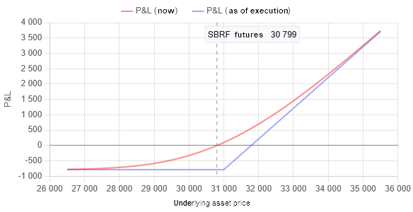
Fig. 1. Dependence of the profit/loss (P&L) of a purchased Call option with a strike of 31,000 on the price of the underlying asset. P&L is expressed in RUB for one option. The vertical dotted line is the moment the graphs were constructed. For this point in time, P&L is negative and equal to -23.92 RUB.

The red line is for the current moment in time (05/22/2025), the blue line is for the expiration time (06/18/2025), i.e. when T = 1 in the Black-Scholes equation

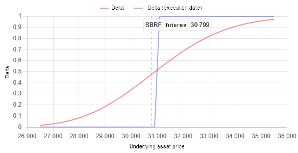
Fig. 2. Dependence of the Delta value of a purchased Call option with a strike of 31,000 on the price of the underlying asset for one option. The vertical dotted line is the moment the graphs were constructed. For this point in time, Delta is 0.48.

The red line is for the current moment in time (05/22/2025), the blue line is for the expiration time (06/18/2025), i.e. when T = 1 in the Black-Scholes equation

The graphs shown above follow directly from the Black-Scholes formula. As can be seen from the graph in Fig. 1, when purchasing a Call option, we pay a premium to the seller in the amount of approximately 789 RUB per contract. In other words, we immediately find ourselves in the red. Unlike an emulated option (the commission for purchasing the underlying asset can, to a first approximation, be neglected). But there is also good news: even if the underlying price falls sharply, the loss is limited to the premium paid. This is the fundamental difference between buying a Call option and buying, for example, a stock - in the latter case, if the price falls, losses are not limited in any way.

We are developing an options emulation in MQL5

Fig. 2 shows that Delta changes (for one contract of a purchased Call option) in the range from 0 to +1. Let's move the X axis of the Delta chart from absolute prices to increments in points. To do this, subtract the strike price from the prices - in this case, 31,000. The resulting graph will look like this:

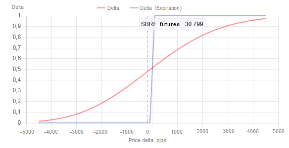
Fig. 3. Dependence of the Delta value of a purchased Call option with a strike of 31,000 on the change in the price of the underlying asset relative to the strike for one option. The vertical dotted line is the moment the graphs were constructed. For this point in time, Delta is 0.48.

The red line is for the current moment in time (05/22/2025), the blue line is for the expiration time (06/18/2025), i.e. when T = 1 in the Black-Scholes equation

Naturally, the resulting graph is qualitatively no different from the original, except for the scale on the X axis. Since the Black-Scholes equation involves implied volatility (IV), which we generally do not know, the only suitable option is to use historical volatility (HV) instead. For monthly options, this will be the average HV for a month, for weekly options, the average HV for a week, etc.

For ease of comparison of charts with different underlying assets and for the possibility of creating options on synthetic instruments (a portfolio consisting of different assets), it would be advisable to use relative price increments, normalizing these increments by the calculated historical volatility.

Then the relative increment from the 'price' is expressed by the following ratio: Relative Price(price) = (price - Strike) / HV.

Let's assume that for the expiration period we calculated HV = 5000. This can be seen in Fig. 3. Obtain a graph of the following type:

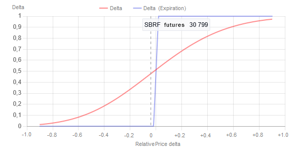
Fig. 4. Dependence of the Delta value of a purchased Call option with a strike of 31,000 on the relative price change, normalized to the historical volatility of the underlying asset for one option. The vertical dotted line is the moment the graphs were constructed. For this point in time, Delta is 0.48.

The red line is for the current moment in time (05/22/2025), the blue line is for the expiration time (06/18/2025), i.e. when T = 1 in the Black-Scholes equation

It can be seen that at a price equal to strike, Delta is equal to 0.5. The delta graph shown by the red line is nothing more than a sigmoid function, known in mathematics and machine learning, of the form: 1 \ (1 + exp(-K \ (x - S))), where S = 0, while K is generally unknown and is selected experimentally. In essence, the K ratio depends on the expiration period. Knowing the value of the delta at a given point in time (0.48) at the current price of the underlying asset (30,800), we can calculate the value of K - for a given point in time it is equal to 2 and will change (increase) as the option approaches expiration.

For the purposes of emulation, we will ignore the time decay of the option and the change of K - it will be constant throughout the option lifetime. This will have a positive effect on the P&L of the purchased Call option and a negative effect on the P&L of the purchased Put option. Overall, there will be no significant impact on the P&L of the options portfolio.

If we equate the S parameter in the sigmoid 1 \ (1 + exp(-K \ (x - S))) to 0.5, then the graph of the dependence of the delta on the relative change in price will shift along the X axis to the right by the S value, and we will get a value at zero that is close to zero - the sigmoid asymptotically tends to 0 and to 1. This type is more convenient for the purposes of emulation and normalization to the volatility range, which we will use when developing an expert in MQL.

So, we have all the source data for writing code in MQL5 to emulate an option on an arbitrary underlying asset. Namely: the equation for the emulation function, the strike price, historical volatility and an understanding of the processes occurring in an ideal Black-Scholes market.

• 1. Base Class

We will emulate the following types of options:

• purchasing the right to buy the underlying asset - Long Call option
• purchasing the right to sell the underlying asset - Long Put option
• selling the right to buy the underlying asset - Short Call option
• selling the right to sell the underlying asset - Short Put option

Let's define all supported option types as an enumeration:

// ---------------------------------------------------------------------
//  Option type:
// ---------------------------------------------------------------------
enum ENUM_OPTION_TYPE
{
   ENUM_OPTION_CALL_LONG,                 // Long Call
   ENUM_OPTION_CALL_SHORT,                // Short Call
   ENUM_OPTION_PUT_LONG,                  // Long Put
   ENUM_OPTION_PUT_SHORT,                 // Short Put
};

The base class is derived from the standard CObject MQL class. This is done to make it easy to use standard MQL CList lists to manipulate objects and create optional constructs of any complexity. This will be discussed in the next article of the series.

The main data members of the base class are:

• option type — type_enum field
• strike price — strike field
• current value of the option delta — delta field
• price for normalizing an option for volatility — norm_price field

There are also a number of auxiliary fields that will be required in classes that descend from the base class. The base class is abstract, with the GetSigmoidValue method required to be defined in descendant classes. This method varies for different types of options within the Black-Scholes model. This approach will also allow for the future addition of other types of options, for example, using machine learning methods and/or other pricing models.

// =====================================================================
// The base class of the option is derived from 'CObject' so that it can be
// put into the lists.
// =====================================================================
class TOptionBase : public CObject
{
protected:
   ENUM_OPTION_TYPE  type_enum;
   double  strike;
   double  shift;
   double  koeff_K;
   double  koeff_S;
   int     digits;
   double  norm_price;
   double  delta;

   double  norm_koeff;
   bool    range_inited_Flag;

public:
   // ---------------------------------------------------------------------
   //  Constructor:
   // ---------------------------------------------------------------------
   TOptionBase(const ENUM_OPTION_TYPE _type, const double _k, const double _s, const int _digits)
   :
   CObject(),
   type_enum(_type),
   strike(0.0),
   shift(0.0),
   koeff_K(_k),
   koeff_S(_s),
   digits(_digits),
   range_inited_Flag(false),
   delta(0.0),
   norm_koeff(0.0)
   {
   }

public:
   // ---------------------------------------------------------------------
   //  Set the delta normalization range for the central strike:
   // ---------------------------------------------------------------------
   void SetRange(const double _strike, const double _norm_price)
   {
     this.strike = _strike;
     this.norm_price = _norm_price;
     this.norm_koeff = 1.0 / (this.norm_price - this.strike);
     this.range_inited_Flag = true;
   }
   // ---------------------------------------------------------------------
   //  Calculate the normalized delta value for a given price:
   // ---------------------------------------------------------------------
   double UpdateDelta(const double _price)
   {
     if(this.range_inited_Flag == false)
     {
       this.delta = 0.0;
     }
     else
     {
       this.delta = NormalizeDouble(this.GetSigmoidValue((_price - this.strike) * this.norm_koeff), 5);
     }

     return(this.delta);
   }
   // ---------------------------------------------------------------------
   //  Get the value of the previously calculated normalized delta:
   // ---------------------------------------------------------------------
   double Delta()
   {
     return(this.delta);
   }
   // ---------------------------------------------------------------------
   //  Get the range initialization flag for the delta:
   // ---------------------------------------------------------------------
   bool    IsRangeInited()
   {
     return(this.range_inited_Flag);
   }
protected:
   // ---------------------------------------------------------------------
   //  Get the normalized delta value:
   // ---------------------------------------------------------------------
   virtual double GetSigmoidValue(const double _x) = 0;
};
// ---------------------------------------------------------------------

• 2. Working in real conditions

When emulating an option, we must choose at what delta change we need to rebalance positions. This will limit the accuracy of the emulation on the one hand, but on the other hand, it will allow us to control the costs of commissions when opening/closing positions. We will use the parameters of the underlying asset - Vmin_size (minimum volume of an open position) and Vmin_delta_size (minimum change in position volume).

We will also set the number of position rebalancings when the delta changes in the range (by modulus) - |0.0...1.0|. We will set this number of rebalancings N as an external parameter. Then the total volume of positions will vary from 0 to (Vmin_size + Vmin_delta_size * (N - 1)).

Typically, Vmin_size is equal to Vmin_deltasize, but this is not necessarily the case. By default, we will take the number of rebalancings equal to ten in the delta range |0.0...1.0|.

• 3. Long Call option

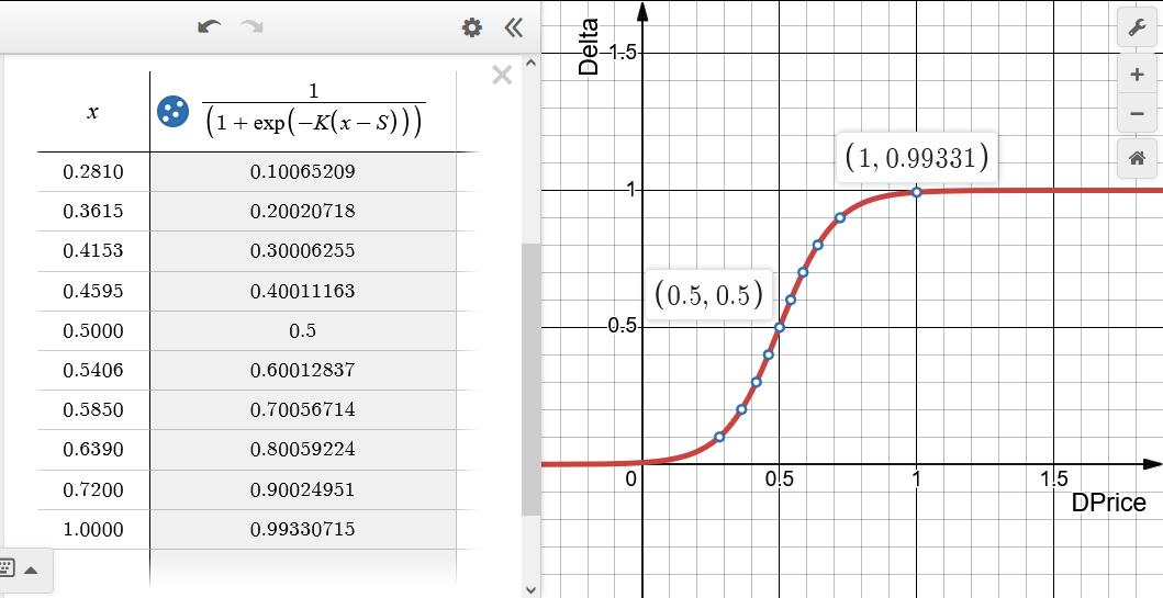
Fig. 5. Dependence of the delta value on the relative change in DPrice (x in the table) for the emulated Long Call option (buying Call). S = 0.5, K = 10. The delta range is divided into ten equal parts

The strike price corresponds to the zero point DPrice = 0. When the delta value is close to one, the option is said to be "deep in the money" - in this case, it behaves like a purchased position on the underlying asset of the maximum size. As the underlying price approaches the strike, the position size in the underlying asset decreases and becomes zero when the option is "out of the money", meaning the delta is close to zero. The real option goes into loss by the amount of the premium.

// =====================================================================
//    Long Call type option class
// =====================================================================
class OptionLongCall : public TOptionBase
{
public:
    // ---------------------------------------------------------------------
    //    Constructor:
    // ---------------------------------------------------------------------
    OptionLongCall(const double _k, const double _s, const int _digits)
    :
    TOptionBase(ENUM_OPTION_CALL_LONG, _k, _s, _digits)
    {
    }

protected:
    // ---------------------------------------------------------------------
    //    Get the normalized delta value:
    // ---------------------------------------------------------------------
    double GetSigmoidValue(const double _x) override
    {
        return(1.0 / (1.0 + MathExp(-this.koeff_K * (_x - this.koeff_S))));
    }
};
// ---------------------------------------------------------------------

• 4. Long Put option

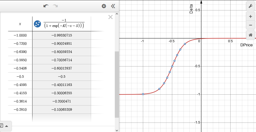
Fig. 6. Dependence of the delta value on the relative change in DPrice (x in the table) for the emulated Long Put option (buying Put). S = 0.5, K = 10. The delta range is divided into ten equal parts

The strike price corresponds to the zero point DPrice= 0. When the delta value is close to minus one, the option is said to be "deep in the money" - in this case, it behaves like a sold position on the underlying asset of the maximum size. As the underlying price approaches the strike, the position size in the underlying asset decreases and becomes zero when the option is "out of the money", meaning the delta is close to zero. The real option goes into loss by the amount of the premium.

// =====================================================================
//    Long Put type option class
// =====================================================================
class OptionLongPut : public TOptionBase
{
public:
    // ---------------------------------------------------------------------
    //    Constructor:
    // ---------------------------------------------------------------------
    OptionLongPut(const double _k, const double _s, const int _digits)
    :
    TOptionBase(ENUM_OPTION_PUT_LONG, _k, _s, _digits)
    {
    }

protected:
    // ---------------------------------------------------------------------
    //    Get the normalized delta value:
    // ---------------------------------------------------------------------
    double GetSigmoidValue(const double _x) override
    {
        return(-1.0 / (1.0 + MathExp(-this.koeff_K * (-_x - this.koeff_S))));
    }
};
// ---------------------------------------------------------------------

• 5. Short Call option

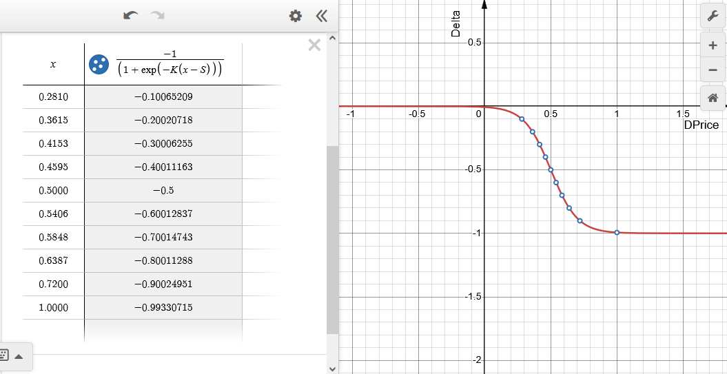
Fig. 7. Dependence of the delta value on the relative change in DPrice (x in the table) for the emulated Short Call option (selling Call). S = 0.5, K = 10. The delta range is divided into ten equal parts

The strike price corresponds to the zero point DPrice= 0. When the delta value is close to minus one, the option is said to be "deep in the money" - in this case, it behaves like a sold position on the underlying asset of the maximum size. As the underlying price approaches the strike, the position size in the underlying asset decreases and becomes zero when the option is "out of the money", meaning the delta is close to zero. The real option goes into profit by the amount of the premium.

// =====================================================================
//    Short Call type option class
// =====================================================================
class OptionShortCall : public TOptionBase
{
public:
    // ---------------------------------------------------------------------
    //    Constructor:
    // ---------------------------------------------------------------------
    OptionShortCall(const double _k, const double _s, const int _digits)
    :
    TOptionBase(ENUM_OPTION_CALL_SHORT, _k, _s, _digits)
    {
    }

protected:
    // ---------------------------------------------------------------------
    //    Get the normalized delta value:
    // ---------------------------------------------------------------------
    double GetSigmoidValue(const double _x) override
    {
        return(-1.0 / (1.0 + MathExp(-this.koeff_K * (_x - this.koeff_S))));
    }
};
// ---------------------------------------------------------------------

• 6. Short Put option

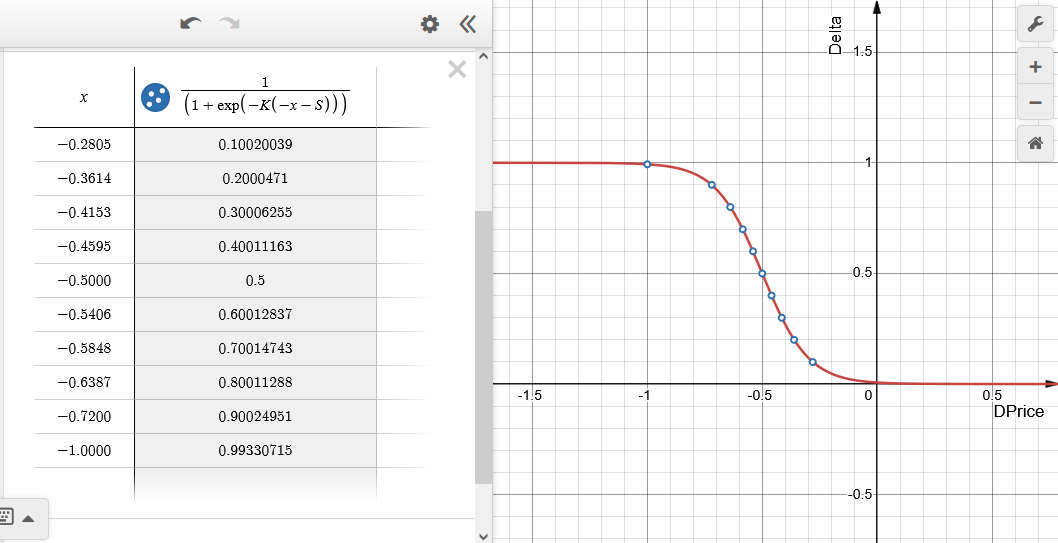
Fig. 8. Dependence of the delta value on the relative change in DPrice (x in the table) for the emulated Short Put option (selling Put). S = 0.5, K = 10. The delta range is divided into ten equal parts

The strike price corresponds to the zero point DPrice= 0. When the delta value is close to one, the option is said to be "deep in the money" - in this case, it behaves like a sold position on the underlying asset of the maximum size. As the underlying price approaches the strike, the position size in the underlying asset decreases and becomes zero when the option is "out of the money", meaning the delta is close to zero. The real option goes into profit by the amount of the premium.

// =====================================================================
//    Short Put type option class
// =====================================================================
class OptionShortPut : public TOptionBase
{
public:
    // ---------------------------------------------------------------------
    //    Constructor:
    // ---------------------------------------------------------------------
    OptionShortPut(const double _k, const double _s, const int _digits)
    :
    TOptionBase(ENUM_OPTION_PUT_SHORT, _k, _s, _digits)
    {
    }

protected:
    // ---------------------------------------------------------------------
    //    Get the normalized delta value:
    // ---------------------------------------------------------------------
    double GetSigmoidValue(const double _x) override
    {
        return(1.0 / (1.0 + MathExp(-this.koeff_K * (-_x - this.koeff_S))));
    }
};
// ---------------------------------------------------------------------

• 7. Peculiarities of calculating the position volume for the underlying asset

To calculate the position volume, we need to convert the delta value from the range |0.0...1.0| to the range of integer values |0...10|. We will then multiply this integer value by the volume of the minimum lot change and obtain the required value of the position volume. 

Let's assume that the number of delta "sub-ranges" is ten. Simply multiplying the delta by ten and converting the result to an integer is insufficient. Since when the delta fluctuates around any boundary of the "sub-range", the volume will also fluctuate synchronously with the delta. Let's explain this with an example: let's say the delta is 0.090 (the volume is then (int)(0.090 * 10) = 0 (i.e. there is no position) and then it grows to 0.101 (the volume is then (int)(0.101 * 10) = 1), then, on the next tick after a short time it decreases again to 0.090 - the volume again becomes equal to 0. That is, we essentially bought and almost immediately sold a position — a meaningless rebalancing of the position that can be repeated many times in a matter of seconds. This is the so-called signal "chattering".

Therefore, when converting the delta to the required volume, there must be a certain "hysteresis" of position rebalancing. This is achieved by distinguishing the direction of rebalancing. We should decrease or increase the current position in the underlying asset and take into account the previous value of the position volume.

Let's introduce the concept of option emulation level. Explanation: if the mapping is set to |0.0...1.0| -> |0...10| (see explanations above), then we will assume that the option emulation level varies from zero to ten. The number of levels is specified as a parameter external to the N parameter. The emulation level, as well as the delta, will be taken modulo. And we will also use the option emulation level sign — {0, +1, -1}. If 0, the position is closed.

• 8. Calculating the position volume for the underlying asset in MQL5

The method for implementing "hysteresis", when calculating the current level of option emulation, is tabular, using two arrays:

• IncreaseLevel_Array — defines the option emulation level when increasing it.
• DecreaseLevel_Array — defines the option emulation level when it is decreased.

This is done in the UpdateOptionLevel method which takes two inputs:

• _delta — option current delta.
• _curr_level — current option emulation level, calculated earlier. Or 0 if this is the first method call.

The OptionContractsVolume class constructor takes two arguments as parameters:

• _ZeroDelta — delta value corresponding to the zero level of option emulation. It may vary from 0.001 to 0.099.
• _LevelsNumber — number of option emulation levels. The more levels, the smoother and more accurate the emulation, but the larger the traded lot in the underlying asset (due to the discreteness of its change).

The constructor populates the IncreaseLevel_Array and DecreaseLevel_Array and various auxiliary variables are initialized (see the source code with comments).

// =====================================================================
//      Class for calculating the contract volume of the underlying asset for an option:
// =====================================================================
class OptionContractsVolume
{
  int IncreaseLevel_Array[];          // option emulation level when increasing it
  int DecreaseLevel_Array[];          // option emulation level when decreasing it
  // ---------------------------------------------------------------------
protected:
  double  ZeroDelta;                  // delta value corresponding to the zero level of option emulation
  int     LevelsNumber;               // number of option emulation levels
  // ---------------------------------------------------------------------
  int     zero_delta;                 // integer delta value corresponding to the zero level of option emulation
  int     curr_option_level_sign;     // current sign of the option emulation level
  int     curr_option_level;          // current option emulation level
  // ---------------------------------------------------------------------
  int     curr_inc_level;
  int     curr_dec_level;
  // ---------------------------------------------------------------------
  int     curr_contracts_index;
  // ---------------------------------------------------------------------
  bool    is_contracts_updated_Flag;

public:
  // ---------------------------------------------------------------------
  //  Constructor:
  // ---------------------------------------------------------------------
  OptionContractsVolume(const double _ZeroDelta, const int _levels_number)
  :
  ZeroDelta(_ZeroDelta),
  LevelsNumber(_levels_number),
  curr_option_level_sign(0),
  curr_option_level(0),
  curr_inc_level(0),
  curr_dec_level(0),
  is_contracts_updated_Flag(false)
  {
    this.zero_delta = (int)(NormalizeDouble(this.ZeroDelta, 3) * 1000.0);

    // Allocate memory for arrays storing emulation levels:
    ArrayResize(this.IncreaseLevel_Array, (this.LevelsNumber + 1) * 100 + 1);
    ArrayResize(this.DecreaseLevel_Array, (this.LevelsNumber + 1) * 100 + 1);

    // Fill in the array upwards:
    for(int i = 0; i < this.LevelsNumber + 1; i++)
    {
      ArrayFill(this.IncreaseLevel_Array, i * this.LevelsNumber * 100, this.LevelsNumber * 100, i);
    }
    ArrayFill(this.IncreaseLevel_Array, (this.LevelsNumber + 1) * 100, 1, this.LevelsNumber);

    // Fill in the array downwards:
    ArrayFill(this.DecreaseLevel_Array, 0,    zero_delta,  0);
    ArrayFill(this.DecreaseLevel_Array, zero_delta,  this.LevelsNumber * 100 - zero_delta + 1,  1);
    for(int i = 2; i < this.LevelsNumber + 1; i++)
    {
      ArrayFill(this.DecreaseLevel_Array, i * this.LevelsNumber * 100,  this.LevelsNumber * 100,  i);
    }
    ArrayFill(this.DecreaseLevel_Array, (this.LevelsNumber + 1) * 100, 1, this.LevelsNumber);
  }
  // ---------------------------------------------------------------------
  //  Calculate the option emulation level for a given delta:
  // ---------------------------------------------------------------------
  //  - if the level has changed, return 'true'.
  // ---------------------------------------------------------------------
  bool  UpdateOptionLevel(const double _delta, const int _curr_level)
  {
    this.is_contracts_updated_Flag = false;

    //  Define trade direction:
    int delta_int = (int)(NormalizeDouble(_delta, 3) * 1000.0);
    this.curr_option_level_sign = 0;
    if(delta_int > zero_delta / 2)
    {
      this.curr_option_level_sign = 1;
    }
    else if(delta_int < -zero_delta / 2)
    {
      this.curr_option_level_sign = -1;
    }

    //  Current index for arrays, based on 'Delta' with 3 decimal places:
    this.curr_contracts_index = (int)MathAbs(delta_int);
    if(this.curr_contracts_index > ((this.LevelsNumber + 1) * 100))
    {
      //  The index should not exceed the array size (here the option is deep in the money):
      this.curr_contracts_index = (this.LevelsNumber + 1) * 100;
    }

    //  Current option emulation level (0...N) in the direction of INCREASE:
    this.curr_inc_level = this.IncreaseLevel_Array[this.curr_contracts_index];

    //  Current option emulation level (0...N) in the direction of DECREASE:
    this.curr_dec_level = this.DecreaseLevel_Array[this.curr_contracts_index];

    //  If the option emulation level (0...N) has INCREASED compared to the current one:
    if(this.curr_inc_level > _curr_level)
    {
      this.curr_option_level = this.curr_inc_level;
      this.is_contracts_updated_Flag = true;
      return(true);
    }

    //  If the option emulation level (0...N) has DECREASED compared to the current one:
    if(this.curr_dec_level < _curr_level)
    {
      this.curr_option_level = this.curr_dec_level;

      this.is_contracts_updated_Flag = true;
      return(true);
    }

    return(false);
  }
};
// ---------------------------------------------------------------------

Find the full code in OptionEmulatorA1.mqh attached below.

Conclusion 

We have considered the emulation of options through the underlying asset. This is a relatively complex and powerful tool that:

• allows creating complex and non-standard option strategies;
• provides more flexibility than standard options;
• requires a deep understanding of mathematical models;
• efficient with proper risk management.

This method is especially useful when we need:

• hedging large portfolios,
• creating exotic option strategies,
• trading in markets with low options liquidity.

Next, we will consider the practical part - maintaining/rebalancing positions in the underlying asset using MQL5 trading functions.