Feature Engineering With Python And MQL5 (Part III): Angle Of Price (2) Polar Coordinates

Open interest in transforming changes in price levels into changes in angles has not slowed down. As we have already discussed in our previous article in this series, there are many challenges to be overcome to successfully convert changes in price levels into an angle that represents that change.

One of the most commonly cited limitations in community discussions and forum posts, is the lack of interpretable meaning behind such calculations. Experienced community members will often explain that an angle exists between two lines, therefore, trying to calculate the angle formed by a change in price has no physical meaning in the real-world. 

The lack of real-world interpretation is just one of the many challenges to be overcome by traders interested in calculating the angle created by changes in price levels. In our previous article, we attempted to solve this problem by substituting time from the x-axis, in order for the angle formed to be a ratio of price levels and have some interpretable meaning. During our exploration, we observed that it is effortless to find our dataset riddled with “infinity” values after performing this transformation. Readers interested in getting a quick refresher of what we observed previously, can find a quick link to the article, here.

Given the numerous challenges that arise when attempting to transform changes in price levels into a corresponding change in angle and the lack of a definite real-world meaning, there is limited, organized information on the subject. 

We will tackle the problem of price to angle conversion from an entirely fresh perspective. This time, we will be using a more mathematically sophisticated and robust approach in comparison to the tools we created on our first attempt. Readers who are already familiar with polar coordinates should feel free to jump straight to the “Getting Started in MQL5” section, to see how these mathematical tools are implemented in MQL5. 

Otherwise, we will now proceed to gain an understanding of what polar coordinates are, and build up an intuition of how we can apply them to calculate the angle formed by price changes on our MetaTrader 5 terminal and use these signals to trade. That is to say:

1. Our proposed solution has real-world physical meaning.
2. We will also satisfy the problem we experienced previously of infinite or undefined values.

What Are Polar Coordinates, And How May They Be Useful?

Whenever we make use of GPS technology or even simple spreadsheets applications, we are employing a technology known as Cartesian Coordinates. This is a mathematical system for representing points in a plane, typically with 2 perpendicular axes. 

Any single point in the Cartesian system is represented as a pair of (x, y) coordinates. Whereby x represents the horizontal distance from the origin, and y represents the vertical distance from the origin. 

If we want to study processes that have periodic components or some form of circular motion, polar coordinates are better suited for this than Cartesian coordinates. Polar coordinates are an entirely different system used to represent points on a plane using a distance from a reference point, and an angle from a reference direction, that increases in an anti-clockwise direction.  

Financial markets tend to demonstrate patterns that repeat, in an almost periodical fashion. Therefore, they may be conformable to be represented as polar coordinates. It appears that, the angle traders desire to calculate from changes in price levels can be naturally obtained by representing price levels as polar pairs. 

Polar coordinates are represented as a pair of (r, theta) whereby:

• R: Represents the radial distance from the reference point (origin)
• Theta: Represents the angle measured from the reference direction.

Using trigonometric functions implemented in the MQL5 Matrix and Vector API, we can seamlessly convert price changes into an angle representing the change in price. 

To achieve our objective, we must first get familiar with the terminology we will use throughout our discussion today. First, we must define our x and y inputs that will be converted. For our discussion, we will set x to be the open price of the Symbol, and y will represent the close price.

Fig 1: Defining our Cartesian points that will be converted to polar points

Now that we have defined our x and y inputs, we need to calculate the first element of the polar pair, the radial distance from the origin, r. 

Fig 2: The closed formula for calculating r, from (x, y)

When represented geometrically, we can imagine polar coordinates as describing a circle. The angle formed between r and x, is theta. Therefore, polar coordinates simply propose that using r and theta is just as informative as using x and y directly. When x and y are envisioned as depicted in Fig 3, then the radial distance, r, is calculated by applying Pythagoras' theorem on sides x and y.

Fig 3: Polar coordinates can be visualized as describing a point on a circle

The angle between r and x, theta, satisfies our desire for real-world meaning. In this simple example, theta correlates to the direction of the trend being formed by changes in the open and close price. Theta is given to us by calculating the inverse tangent of the close price divided by the open price, as depicted in Fig below.

Fig 4: Calculating theta from our Open (x) and Close (y) price

Given any polar coordinates (r, theta), we can easily convert them back into their original price levels using the 2 formulas below:

Fig 5: How to convert Polar coordinates back into Cartesian coordinates

We have discussed 4 formulas so far, but only the last 3 formulas contain theta. The first formula that we use to calculate r has no relation to theta. The last 3 formulas we have discussed contain theta and can easily be differentiated. The derivatives of these trigonometric functions are well-known results that can be easily found online or in any elementary calculus textbook. 

We will use these 3 derivatives as additional inputs to train our computer to learn the relationship between changes in angles and their corresponding changes in price levels.

Getting Started In MQL5

Let us get started. We first need to build a script in MQL5 that will fetch historical market data from our MetaTrader 5 Terminal, and also perform the transformations to give us the angles being created.

We first need to define the name of the CSV file we are creating, and then also specify how many bars of data to fetch. Since the number of bars to fetch may vary depending on your broker, we have set this parameter to be an input for the script.

#property copyright "Gamuchirai Zororo Ndawana"
#property link      "https://www.mql5.com"
#property version   "1.00"
#property script_show_inputs

//---File name
string file_name = _Symbol + " " + " Polar Coordinates.csv";

//---Amount of data requested
input int size = 100;
int size_fetch = size + 100;

When our script is executed, we will create a file handler to write out the price levels and their corresponding changes in angle.

void OnStart()
  {
      //---Write to file
       int file_handle=FileOpen(file_name,FILE_WRITE|FILE_ANSI|FILE_CSV,",");
       
    for(int i=size;i>0;i--){
      if(i == size){
            FileWrite(file_handle,"Time","Open","High","Low","Close","R","Theta","X Derivatie","Y Derivative","Theta Derivative");
      }
      
      else{

Let us proceed to calculate r using the formula we discussed in Fig 2.

double r = MathSqrt(MathPow(iOpen(_Symbol,PERIOD_CURRENT,i),2) + MathPow(iClose(_Symbol,PERIOD_CURRENT,i),2));

Theta is calculated through inverse tan of the ratio between y and x. This is implemented for us in the MQL5 API.

double theta = MathArctan2(iClose(_Symbol,PERIOD_CURRENT,i),iOpen(_Symbol,PERIOD_CURRENT,i));

Recall that the formula for calculating x (Open price), is provided in Fig 5 above. We can differentiate this formula regarding theta to calculate the first derivative of the open price. The derivative of cos(), as you know already, is -sin().

double derivative_x = r * (-(MathSin(theta)));

We can also calculate the derivative of y since we know the derivative of trigonometric functions.

double derivative_y = r * MathCos(theta);

Lastly, we know the first derivative of theta. However, the trig function is not directly implemented in the MQL5 API, rather we will use a mathematical identity to substitute it using the appropriate MQL5 functions.

double derivative_theta = (1/MathPow(MathCos(theta),2));

Now that we have calculated our angles, we can proceed to write out our data.

           FileWrite(file_handle,iTime(_Symbol,PERIOD_CURRENT,i),
                                 iOpen(_Symbol,PERIOD_CURRENT,i),
                                 iHigh(_Symbol,PERIOD_CURRENT,i),
                                 iLow(_Symbol,PERIOD_CURRENT,i),
                                 iClose(_Symbol,PERIOD_CURRENT,i),
                                 r,
                                 theta,
                                 derivative_x,
                                 derivative_y,
                                 derivative_y
                                 );
      } 
    }
    
    FileClose(file_handle);
  }
//+---------

Analyzing Our Data

Now that our data is written out in CSV format, let's use it to train our computer to trade the angles formed. We will be using a few Python libraries to accelerate our development process.

import pandas as pd
import numpy as np
import seaborn as sns
import matplotlib.pyplot as plt

Label the data to note if price levels increased the following day, or if they fell the following day.

data = pd.read_csv("EURUSD  Polar Coordinates.csv")
data["UP DOWN"] = 0
data.loc[data["Close"] < data["Close"].shift(-1),"UP DOWN"] = 1
data

Here is the trading signal we are looking for. Note that whenever R and Theta both increase in our original dataset, price levels never fall. This call to pandas returns nothing, and this shows the real-world meaning backing polar pairs. Knowing the future values of R and Theta, is just as good as knowing the future price level.

data.loc[(data["R"] < data["R"].shift(-1)) & (data['Theta'] < data['Theta'].shift(-1)) & (data['Close'] > data['Close'].shift(-1))

Likewise, if we perform the same query but in the opposite direction, that is to say, we are looking for instances where R and Theta increased, but the future price fell, again we will find pandas returns 0 instances.

data.loc[(data["R"] > data["R"].shift(-1)) & (data['Theta'] > data['Theta'].shift(-1)) & (data['Close'] < data['Close'].shift(-1))]

Therefore, our trading signals will be formed whenever our computer expects the future values of R and Theta to be greater than their current values. Moving on, we can now visualize our price data as points on a polar circle. As we can observe in Fig 6, the data is still challenging to separate effectively.

data['Theta_rescaled'] = (data['Theta'] - data['Theta'].min()) / (data['Theta'].max() - data['Theta'].min()) * (2 * np.pi)
data['R_rescaled'] = (data['R'] - data['R'].min()) / (data['R'].max() - data['R'].min()) 

# Create the polar plot
fig, ax = plt.subplots(subplot_kw={'projection': 'polar'})

# Plot data points on the polar axis
ax.scatter(data['Theta_rescaled'], data['R_rescaled'],c=data["UP DOWN"], cmap='viridis', edgecolor='black', s=100)

# Add plot labels
ax.set_title("Polar Plot of OHLC Points")
plt.colorbar(plt.cm.ScalarMappable(cmap='viridis'), ax=ax, label='1(UP) | O(DOWN)')

plt.show()

Fig 6: Visualizing our price data as polar points on a polar circle

Let us quickly check if any of our values are null.

data.isna().any()

Fig 7: Checking if any of our values are null

Modelling The Data

All our values are defined, great. We also need to label the data. Recall that our target is the future value of theta and r.

LOOK_AHEAD = 1
data['R Target'] = data['R'].shift(-LOOK_AHEAD)
data['Theta Target'] = data['Theta'].shift(-LOOK_AHEAD)
data.dropna(inplace=True)
data.reset_index(drop=True,inplace=True)

Keep in mind, we want to drop the last 2 years of data so we can use them as our test for our application.

#Let's entirely drop off the last 2 years of data
_ = data.iloc[-((365 * 2) + 230):,:]
data = data.iloc[:-((365 * 2) + 230),:]
data

Fig 8: Our dataset after dropping off the last 2 years of data

Let us now train the computer using the data on hand. We will use a gradient boosted tree as our model of choice because they are particularly good at learning interaction effects.

from sklearn.ensemble import GradientBoostingRegressor
from sklearn.model_selection import train_test_split,TimeSeriesSplit,cross_val_score

Now define our time series split object.

tscv = TimeSeriesSplit(n_splits=5,gap=LOOK_AHEAD)

Define the inputs and targets.

X = data.columns[1:-5]
y = data.columns[-2:]

Partition the data into training and testing halves.

train , test = train_test_split(data,test_size=0.5,shuffle=False)

Now prepare the train, test splits.

train_X = train.loc[:,X]
train_y = train.loc[:,y]

test_X = test.loc[:,X]
test_y = test.loc[:,y]

The training and testing splits need to be standardized.

mean_scores = train_X.mean()
std_scores = train_X.std()

Scaling the data.

train_X = ((train_X - mean_scores) / std_scores)
test_X = ((test_X - mean_scores) / std_scores)

Initialize the model.

model = GradientBoostingRegressor()

Prepare a table to store the results.

results = pd.DataFrame(index=["Train","Test"],columns=["GBR"])

Fit the model to predict R.

results.iloc[0,0] = np.mean(np.abs(cross_val_score(model,train_X,train_y["R Target"],cv=tscv)))
results.iloc[1,0] = np.mean(np.abs(cross_val_score(model,test_X,test_y["R Target"],cv=tscv)))
results

GBR
Train	0.76686
Test	0.89129

Fit the model to Predict Theta.

results.iloc[0,0] = np.mean(np.abs(cross_val_score(model,train_X,train_y["Theta Target"],cv=tscv)))
results.iloc[1,0] = np.mean(np.abs(cross_val_score(model,test_X,test_y["Theta Target"],cv=tscv)))
results

GBR
Train	0.368166
Test	0.110126

Exporting To ONNX

Load the libraries we need.

import onnx
import skl2onnx 
from skl2onnx.common.data_types import FloatTensorType

Initialize the models.

r_model = GradientBoostingRegressor()
theta_model = GradientBoostingRegressor()

Store the global standardization scores for the entire dataset to CSV format.

mean_scores = data.loc[:,X].mean()
std_scores = data.loc[:,X].std()

mean_scores.to_csv("EURUSD Polar Coordinates Mean.csv")
std_scores.to_csv("EURUSD Polar Coordinates Std.csv")

Normalize the entire dataset.

data[X] = ((data.loc[:,X] - mean_scores) / std_scores)

Fit the models on the scaled data.

r_model.fit(data.loc[:,X],data.loc[:,'R Target'])
theta_model.fit(data.loc[:,X],data.loc[:,'Theta Target'])

Define the input shape.

initial_types = [("float_input",FloatTensorType([1,len(X)]))]

Prepare the ONNX prototypes to be saved.

r_model_proto = skl2onnx.convert_sklearn(r_model,initial_types=initial_types,target_opset=12)
theta_model_proto = skl2onnx.convert_sklearn(theta_model,initial_types=initial_types,target_opset=12)

Save the ONNX files.

onnx.save(r_model_proto,"EURUSD D1 R Model.onnx")
onnx.save(theta_model_proto,"EURUSD D1 Theta Model.onnx")

Getting Started In MQL5

We are now ready to build our trading application.

//+------------------------------------------------------------------+
//|                                              EURUSD Polar EA.mq5 |
//|                                               Gamuchirai Ndawana |
//|                    https://www.mql5.com/en/users/gamuchiraindawa |
//+------------------------------------------------------------------+
#property copyright "Gamuchirai Ndawana"
#property link      "https://www.mql5.com/en/users/gamuchiraindawa"
#property version   "1.00"

//+------------------------------------------------------------------+
//| System Constants                                                 |
//+------------------------------------------------------------------+
#define ONNX_INPUTS 9                                              //The total number of inputs for our onnx model
#define ONNX_OUTPUTS 1                                             //The total number of outputs for our onnx model
#define TF_1  PERIOD_D1                                            //The system's primary time frame
#define TRADING_VOLUME 0.1                                         //The system's trading volume

Load the ONNX models as system resources.

//+------------------------------------------------------------------+
//| System Resources                                                 |
//+------------------------------------------------------------------+
#resource "\\Files\\EURUSD D1 R Model.onnx" as uchar r_model_buffer[];
#resource "\\Files\\EURUSD D1 Theta Model.onnx" as uchar theta_model_buffer[];

Define our global variables. We will use some of these variables to standardize our data, store our ONNX model's forecasts and much more.

//+------------------------------------------------------------------+
//| Global variables                                                 |
//+------------------------------------------------------------------+
double mean_values[] = {1.1884188643844635,1.1920754015799868,1.1847545720868993,1.1883860236998025,1.6806588395310122,0.7853854898794739,-1.1883860236998025,1.1884188643844635,1.1884188643844635};
double std_values[]  = {0.09123896995032886,0.09116171300874902,0.0912656190371797,0.09120265318308786,0.1289537623737421,0.0021932437785043796,0.09120265318308786,0.09123896995032886,0.09123896995032886};
double current_r,current_theta;
long r_model,theta_model;
vectorf r_model_output = vectorf::Zeros(ONNX_OUTPUTS);
vectorf theta_model_output = vectorf::Zeros(ONNX_OUTPUTS);
double bid,ask;
int ma_o_handler,ma_c_handler,state;
double ma_o_buffer[],ma_c_buffer[];

Load the trade library.

//+------------------------------------------------------------------+
//| Library                                                          |
//+------------------------------------------------------------------+
#include <Trade/Trade.mqh>
CTrade Trade;

Our trading application is mainly composed of event handlers. During each stage of the application's life cycle, we will call dedicated functions to perform tasks that correspond to our objective at that time. So during initialization, we will set up our technical indicators, and when new prices are available, we will update our readings from those indicators.

//+------------------------------------------------------------------+
//| Expert initialization function                                   |
//+------------------------------------------------------------------+
int OnInit()
  {
//---
   if(!setup())
     {
      Comment("Failed To Load Corretly");
      return(INIT_FAILED);
     }

   Comment("Started");
//---
   return(INIT_SUCCEEDED);
  }
//+------------------------------------------------------------------+
//| Expert deinitialization function                                 |
//+------------------------------------------------------------------+
void OnDeinit(const int reason)
  {
//---
   OnnxRelease(r_model);
   OnnxRelease(theta_model);
  }
//+------------------------------------------------------------------+
//| Expert tick function                                             |
//+------------------------------------------------------------------+
void OnTick()
  {
//---
   update();
  }
//+------------------------------------------------------------------+

Getting a prediction from our ONNX model. Note that, we type cast all the model inputs to the float type, to ensure that the model receives data of the right format and size, given its expectations.

//+------------------------------------------------------------------+
//| Get a prediction from our models                                 |
//+------------------------------------------------------------------+
void get_model_prediction(void)
  {
//Define theta and r
   double o = iOpen(_Symbol,PERIOD_CURRENT,1);
   double h = iHigh(_Symbol,PERIOD_CURRENT,1);
   double l = iLow(_Symbol,PERIOD_CURRENT,1);
   double c = iClose(_Symbol,PERIOD_CURRENT,1);
   current_r = MathSqrt(MathPow(o,2) + MathPow(c,2));
   current_theta = MathArctan2(c,o);

   vectorf model_inputs =
     {
      (float) o,
      (float) h,
      (float) l,
      (float) c,
      (float) current_r,
      (float) current_theta,
      (float)(current_r * (-(MathSin(current_theta)))),
      (float)(current_r * MathCos(current_theta)),
      (float)(1/MathPow(MathCos(current_theta),2))
     };

//Standardize the model inputs
   for(int i = 0; i < ONNX_INPUTS;i++)
     {
      model_inputs[i] = (float)((model_inputs[i] - mean_values[i]) / std_values[i]);
     }

//Get a prediction from our model
   OnnxRun(r_model,ONNX_DATA_TYPE_FLOAT,model_inputs,r_model_output);
   OnnxRun(theta_model,ONNX_DATA_TYPE_FLOAT,model_inputs,theta_model_output);

//Give our prediction
   Comment(StringFormat("R: %f \nTheta: %f\nR Forecast: %f\nTheta Forecast: %f",current_r,current_theta,r_model_output[0],theta_model_output[0]));
  }

Update the system whenever new prices are offered.

//+------------------------------------------------------------------+
//| Update system state                                              |
//+------------------------------------------------------------------+
void update(void)
  {
   static datetime time_stamp;
   datetime current_time = iTime(_Symbol,TF_1,0);

   bid = SymbolInfoDouble(_Symbol,SYMBOL_BID);
   ask = SymbolInfoDouble(_Symbol,SYMBOL_ASK);
   if(current_time != time_stamp)
     {
      CopyBuffer(ma_o_handler,0,0,1,ma_o_buffer);
      CopyBuffer(ma_c_handler,0,0,1,ma_c_buffer);
      time_stamp = current_time;
      get_model_prediction();
      manage_account();
      if(PositionsTotal() == 0)
         get_signal();
     }
  }

Manage the account. If we are loosing money on a trade, we would rather close it promptly. Otherwise, if we have entered into a trade, but the moving averages cross over in a way the undermines our confidence in that position, we will close it right away.

//+------------------------------------------------------------------+
//| Manage the open positions we have in the market                  |
//+------------------------------------------------------------------+
void manage_account()
  {
   if(AccountInfoDouble(ACCOUNT_BALANCE) < AccountInfoDouble(ACCOUNT_EQUITY))
     {
      while(PositionsTotal() > 0)
         Trade.PositionClose(Symbol());
     }

   if(state == 1)
     {
      if(ma_c_buffer[0] < ma_o_buffer[0])
         Trade.PositionClose(Symbol());
     }

   if(state == -1)
     {
      if(ma_c_buffer[0] > ma_o_buffer[0])
         Trade.PositionClose(Symbol());
     }
  }

Setup system variables, such as technical indicators and ONNX models.

//+------------------------------------------------------------------+
//| Setup system variables                                           |
//+------------------------------------------------------------------+
bool setup(void)
  {
   ma_o_handler = iMA(Symbol(),TF_1,50,0,MODE_SMA,PRICE_CLOSE);
   ma_c_handler = iMA(Symbol(),TF_1,10,0,MODE_SMA,PRICE_CLOSE);

   r_model = OnnxCreateFromBuffer(r_model_buffer,ONNX_DEFAULT);
   theta_model = OnnxCreateFromBuffer(theta_model_buffer,ONNX_DEFAULT);

   if(r_model == INVALID_HANDLE)
      return(false);
   if(theta_model == INVALID_HANDLE)
      return(false);

   ulong input_shape[] = {1,ONNX_INPUTS};
   ulong output_shape[] = {1,ONNX_OUTPUTS};

   if(!OnnxSetInputShape(r_model,0,input_shape))
      return(false);
   if(!OnnxSetInputShape(theta_model,0,input_shape))
      return(false);

   if(!OnnxSetOutputShape(r_model,0,output_shape))
      return(false);
   if(!OnnxSetOutputShape(theta_model,0,output_shape))
      return(false);

   return(true);
  }

Check if we have a trading signal. We will primarily check the orientation of our moving average cross over strategy. Afterward, we will check our expectations given to us by the ONNX models. Therefore, if the moving average cross over gives us bearish sentiment, but our r and theta ONNX models give us bullish sentiment, we will not open any positions until the 2 systems are in agreement.

//+------------------------------------------------------------------+
//| Check if we have a trading signal                                |
//+------------------------------------------------------------------+
void get_signal(void)
  {
   if(ma_c_buffer[0] > ma_o_buffer[0])
     {
      if((r_model_output[0] < current_r) && (theta_model_output[0] < current_theta))
        {
         return;
        }
        
      if((r_model_output[0] > current_r) && (theta_model_output[0] > current_theta))
        {
         Trade.Buy(TRADING_VOLUME * 2,Symbol(),ask,0,0);
         Trade.Buy(TRADING_VOLUME * 2,Symbol(),ask,0,0);
         state = 1;
         return;
        }
        
      Trade.Buy(TRADING_VOLUME,Symbol(),ask,0,0);
      state = 1;
      return;
     }

   if(ma_c_buffer[0] < ma_o_buffer[0])
     {
      if((r_model_output[0] > current_r) && (theta_model_output[0] > current_theta))
        {
         return;
        }

     if((r_model_output[0] < current_r) && (theta_model_output[0] < current_theta))
        {
         
         Trade.Sell(TRADING_VOLUME * 2,Symbol(),bid,0,0);
         Trade.Sell(TRADING_VOLUME * 2,Symbol(),bid,0,0);
         state = -1;
         return;
        }

      Trade.Sell(TRADING_VOLUME,Symbol(),bid,0,0);
      state = -1;
      return;
     }
  }

Undefine system constants we aren't using.

//+------------------------------------------------------------------+
//| Undefine system variables we don't need                          |
//+------------------------------------------------------------------+
#undef ONNX_INPUTS
#undef ONNX_OUTPUTS
#undef TF_1
//+------------------------------------------------------------------+

Testing Our System

Let us now start testing our system. Recall that during our data preparation step, we dropped the data from 1 January 2022, so that our back test reflects how well our strategy could perform on data it has not seen, ever.

Fig 9: Our back test settings

Now specify the initial account settings. 

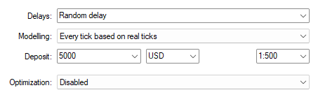
Fig 10: Our second batch of settings for our crucial back test over out of sample data

We can observe the equity curve of the trading signals produced by our new system. Our strategy started with a balance of $5000 and finished with a balance of around $7000, these are good results and encourage us to keep exploring and redefining our strategy.

Fig 11: The back test results we obtained from trading the signals generated by our angle transformations

Let us analyze our results in detail. Our strategy had an accuracy of 88% on out of sample data. This is encouraging information, and may render the reader a good starting place to build their own applications by extending the functionality and capability of the MetaTrader 5 Terminal we have demonstrated in this application. Or the reader may consider using our framework as a guide instead, and entirely replacing our trading strategy, with their own.

Fig 12: Analyzing the results of our back test in detail

Conclusion

The solution we have provided you today have demonstrated to you how to realize the potential edge found by meaningfully converting changes in price levels into changes in angles. Our procedure provides you with a simple and elegant framework for tackling this issue, allowing you to have the best blend of both trading logic and mathematical logic. Moreover, unlike casual market participants that are stuck trying to predict price directly, you now have alternative targets that are just as useful as knowing price itself while being easier to predict consistently than price itself.

Attached File	Description
Polar Fetch Data	Our customized script for fetching our price data and transforming it into polar coordinates.
EURUSD Polar EA	The Expert Advisor that trades the signals generated from the changes in angle detected.
EURUSD D1 R Model	The ONNX model responsible for predicting our future values of R
EURUSD D1 Theta Model	The ONNX model responsible for predicting our future values of Theta
EURUSD Polar Coordinates	The Jupyter Notebook we used to analyze the data we fetched with our MQL5 script