MQL5 Wizard Techniques you should know (Part 12): Newton Polynomial

Introduction

Time series analysis plays an important role not just in supporting fundamental analysis but in very liquid markets like forex, it can be the main driver for decisions on how one is positioned in the markets. Traditional technical indicators have tended to lag the market a lot which has brought them out of favor for most traders, leading to the rise of alternatives perhaps the most predominant of which, at the moment is neural networks. But what about polynomial interpolation?

Well they present some advantages mainly from being easy to understand and implement since they explicitly present the relationship between past observations and future forecasts in a simple equation. This helps in understanding how past data impacts future values which in turn leads to developing broad concepts and possible theories on the studied time series’ behavior.

In addition, being adaptable to both linear and quadratic relations make them flexible to various time series and perhaps more pertinent for traders, capable of coping in different market types (e.g. ranging vs trending or volatile vs calm markets)

Furthermore, they are typically not compute-intense and are relatively lightweight when compared to alternative approaches like neural networks. In fact, the model(s) examined in this article have zero storage requirements the kind you would need with say a neural network where depending on its architecture where making provision for storing a lot the optimal weights and biases after each training session is a requirement.

So, formally newton’s interpolation polynomial N(x) is defined by the equation:

where all x j are unique in the series and a j is the sum of divided differences while n j (x) is the product sum of the basis coefficients for x that is formally represented as follows:

The divided differences and basis coefficients formulae can easily be looked up independently however let’s try to unpack their definitions here as informally as possible.

Divided differences are a repetitive division process that sets coefficients for x at each exponent until all x exponents are exhausted from the provided data set. To illustrate this let’s consider the sample below of three data points:

(1,2), (3,4), and (5,6)

For divided difference to be used all x values need to be unique. The number of provided data points infer the highest exponent of x in the newton form polynomial that gets derived. If we had only 2 points for instance then our equation would simply be linear in the form:

y = mx + c.

Implying our highest exponent is one. For our three-point example therefore the highest exponent is 2 meaning we need to get 3 different coefficients for our derived polynomial.

Getting each of these 3 coefficients is a step by step, iterative process until we arrive at the third. There are formulae in the links shared above, but probably the best way to understand this would be by using a table such as the one shown below:

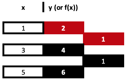
So, our first column of divided differences is got from dividing the difference between the y values and the change in the respective x values. Remember all x values need to be unique. These computations are very simple and straight forward however they are easy to follow from a table as shown above rather than the typical formulae referred to in the shared links. Both approaches lead to the same result.

= (4 - 2) / (3 - 1)

Gives us our first coefficient, 1.

= (6 - 4) / (5 - 3)

Gives us the second coefficient of simillar value. Coefficients are highlighted in red.

From our 3 data point example the final value would get its y differences from the just computed values but its x denominators

would be the two extreme values in the x series as their difference will be the divisor so our table would complete as follows:

With our completed table above, we have 3 derived values but only 2 of them are used in getting the coefficients. This thus leads us to the product sums of the “basis polynomials”. As fancy as it sounds, its really straight forward in fact more so than even the divided differences. So, to illustrate this, based on our derived coefficients from the table above, our equation for the three points would be:

y = 2 + 1*(x – 1) + 0*(x – 1)*(x – 3)

this comes to:

y = x + 1

The added brackets are all that constitutes the basis polynomials. The x n value simply being the respective x value for each sampled data point. Now back to the coefficients and you’ll note that as a rule we only use the top values of the table in prefixing these bracket values and as we progress to the right by getting shorter columns in the table, top values prefix longer bracket sequences until all provided data points are considered. As mentioned the more data points to interpolate, the more exponents of x and thus the more columns we will have in our deriving table.

Let us have one more engaging illustration of this before moving on to implementation. Supposing we have 7 data points for security prices where x values are simply the price bar index as shown below:

0	1.25590
1	1.26370
2	1.25890
3	1.25395
4	1.25785
5	1.26565
6	1.26175

Our table that propagates the coefficient values would extend out by 8 columns as follows:

<table: 8 columns of divided differences />

With the coefficients highlighted in red, the equation from this would therefore be as follows:

y = 1.2559 + 0.0078*(x – 0) – 0.0063*(x – 0)*(x – 1) + …

This equation as is evident goes up to the exponent 6, given the seven data points and arguably its key function could be in forecasting the next value by inputting a new x index into the equation. If the sampled data was ‘set as a series’ then the next index would be -1 otherwise it would be 8.

MQL5 Implementation:

Implementing this in MQL5 can be achieved with minimal coding although it could be worth mentioning I was not able to come across any libraries that allow these ideas to be run from pre-coded class instances, for example.

To have this though, we need to do basically two things. First, we need a function to work out the coefficients to x for our equation given our sampled data set. Secondly, we also need a function to process a forecast value using our equation when presented with an x value. It all sounds pretty straight forward but considering we want to do this in a scalable manner, it does require being mindful of a few caveats in the processing steps.

So, perhaps before we get into it, what is implied by ‘scalable manner’? By this am simply referring to functions that can use divided differences to come up with coefficients for data sets whose size is not predetermined. It may sound obvious but if we consider our very first 3 data point example, the MQL5 implementation of this to get the coefficients is:

<code: solving coefficients for 3 points />

The above listing simply follows equations for getting the divided difference for the two pairs within the sampled data and iterates this procedure to also get the last value. Now if we were to have a 4 data point sample then interpolating its equation would require a different function since we have more steps to make than those shown in the 3-point example above.

So, if we have a scalable function it would be capable of handling n sized datasets and outputting n-1 coefficients. This is realized by the following listing:

//+------------------------------------------------------------------+
//| INPUT PARAMETERS                                                 |
//|     X   -   vector with x values of sampled data                 |
//|     Y   -   vector with y values of sampled data                 |
//| OUTPUT PARAMETERS                                                |
//|     W   -   vector with coefficients.                            |                                          |
//+------------------------------------------------------------------+
void Cnewton::Set(vector &W, vector &X, vector &Y)
{  vector _w[];
   ArrayResize(_w, int(X.Size() - 1));
   int _x_scale = 1;
   int _y_scale = int(X.Size() - 1);
   for(int i = 0; i < int(X.Size() - 1); i++)
   {  _w[i].Init(_y_scale);
      for(int ii = 0; ii < _y_scale; ii++)
      {  if(X[ii + _x_scale] != X[ii])
         {  if(i == 0)
            {  _w[i][ii] = (Y[ii + 1] - Y[ii]) / (X[ii + _x_scale] - X[ii]);
            }
            else if(i > 0)
            {  _w[i][ii] = (_w[i - 1][ii + 1] - _w[i - 1][ii]) / (X[ii + _x_scale] - X[ii]);
            }
         }
         else
         {  printf(__FUNCSIG__ + " ERR!, identical X value: " + DoubleToString(X[ii + _x_scale]) + ", at: " + IntegerToString(ii + _x_scale) + ", and: " + IntegerToString(ii));
            return;
         }
      }
      _x_scale++;
      _y_scale--;
      W[i + 1] = _w[i][0];
      if(_y_scale <= 0)
      {  break;
      }
   }
}

This function operates by using two nested for loops and two integers that track indices for x and y values. It may not be the most efficient way to implement this but it works and absent of a standard library that implements this I would encourage exploring it and even making improvements to it depending one’s use case.

The function for processing the next y given an x input and all our equations coefficients is also shared below:

//+------------------------------------------------------------------+
//| INPUT PARAMETERS                                                 |
//|     W   -   vector with pre-computed coefficients                |
//|     X   -   vector with x values of sampled data                 |
//|     XX  -   query x value with unknown y                         |
//| OUTPUT PARAMETERS                                                |
//|     YY  -   solution for unknown y.                              |  
//+------------------------------------------------------------------+
void Cnewton::Get(vector &W, vector &X, double &XX, double &YY)
{  YY = W[0];
   for(int i = 1; i < int(W.Size()); i++)
   {  double _y = W[i];
      for(int ii = 0; ii < i; ii++)
      {  _y *= (XX - X[ii]);
      }
      YY += _y;
   }
}

This is also more straight forward than our prior function even though it also has a nested loop all we are doing is tracking the coefficients we obtained in the set function and assigning them to their appropriate Newton-basis-polynomial.

Applications:

Applications of this can be wide ranging and for this article we will consider how this can be of use as a signal, a trailing stop method, and a money management method. Before these are coded it’s normally a good idea to have an anchor class with the two functions, implementing the interpolation, whose code is listed above. For such a class we’ll have its interface as follows:

//+------------------------------------------------------------------+
//|                                                                  |
//+------------------------------------------------------------------+
class Cnewton
{
private:

public:
                     Cnewton();
                    ~Cnewton();
   void              Set(vector &W, vector &X, vector &Y);
   void              Get(vector &W, vector &X, double &XX, double &YY);
};

Signal

The standard expert signal class files provided in the MQL5 library as always serve as a healthy guide on developing one’s custom implementation. In our case the first obvious choice for input sample data, to generate the polynomial, would be raw security close prices. To generate a polynomial based off close prices we would first fill the x and y vectors with price bar indices and actual close prices respectively. These two vectors are the key inputs of our ‘set’ function that is responsible for getting the coefficients. On a side note we are simply using price bar indices for x in our signal but is possible to use alternatives such as the sessions in a trade day, or in a trade week, provided of course none of these are repeated in the data sample i.e. they all only appear once e.g. if your trade day has 4 sessions then you can provide no more than 4 data points and the session indices 0, 1, 2, & 3 can only appear once within the data set.

After filling our x and y vectors, calling the ‘set’ function should provide the preliminary coefficients to our polynomial equation. If we run this equation with these coefficients and the next x value using the ‘get’ function we get the projection for what the next y value will be. Since our input y values in the set function were close prices, we’d be looking to get the next close price. The code for this is shared below:

<code: check open long up to calling ‘get’ />

In addition to getting the next projected close price the check open functions of the expert signal class typically output an integer that is in the range of 0 – 100 as a sign of how strong the buy or sell signal is. In our case therefore we need to find a way of representing the projected close price as a simple integer that fits in this range.

To get this normalization, the projected close price change is expressed as a percentage of the current high – low price range. This percentage is then expressed as an integer in the 0 – 100 range. This implies that negative close price changes in the ‘check for open long’ function will automatically be zero, and so will positive forecast changes in the ‘check for open short’ function.

<code: check open long normalization end… />

In making forecasts via the polynomial equation the only variable we are using is the length of the look back period (which sets the sampling data size). This variable is labelled ‘m_length’. If we run optimizations for only this parameter for the symbol EURJPY on the 1-hour time frame over the year 2023, we get the following reports.

A complete run over the whole year gives us this equity picture:

Trailing-Stop

Besides the expert signal class, we can assemble an expert adviser with the wizard by also selecting a method for setting and adjusting the trailing stop of open positions. Provided within the library are methods that use Parabolic Sar and moving averages and on the whole their number is much less than what is in the signal library. If we are to improve this count by adding a class that uses newton’s polynomial, then arguably our sampled data would have to be price bar ranges.

If we therefore follow the same steps we took above when projecting the next close price, with the main change being data to the y vector which in this case will now be price bar ranges, then our source would be as follows:

//+------------------------------------------------------------------+
//| Checking trailing stop and/or profit for long position.          |
//+------------------------------------------------------------------+
bool CTrailingNP::CheckTrailingStopLong(CPositionInfo *position, double &sl, double &tp)
{
//--- check

   ...

//---
   m_high.Refresh(-1);
   m_low.Refresh(-1);
   vector _x, _y;
   _x.Init(m_length);
   _y.Init(m_length);
   for(int i = 0; i < m_length; i++)
   {  _x[i] = i;
      _y[i] = (m_high.GetData(StartIndex()+i)-m_low.GetData(StartIndex()+i));
   }
   vector _w;
   _w.Init(m_length);
   _w[0] = _y[0];
   __N.Set(_w, _x, _y);
   double _xx = -1.0;
   double _yy = 0.0;
   __N.Get(_w, _x, _xx, _yy);
//---

   ...

//---
   return(sl != EMPTY_VALUE);
}

A proportion of this forecast bar range is then used to set the size of the position stop loss. The proportion used is an optimizable parameter ‘m_stop_level’ and before the new stop loss is set we add the minimum stop distance to this delta to avoid any broker errors. This normalization is captured by the code below:

//+------------------------------------------------------------------+
//| Checking trailing stop and/or profit for long position.          |
//+------------------------------------------------------------------+
bool CTrailingNP::CheckTrailingStopLong(CPositionInfo *position, double &sl, double &tp)
{
//--- check
   
   ...

//---
   sl = EMPTY_VALUE;
   tp = EMPTY_VALUE;
   delta = (m_stop_level * _yy) + (m_symbol.Point() * m_symbol.StopsLevel());
//---
   if(price - base > delta)
   {  sl = price - delta;
   }
//---
   return(sl != EMPTY_VALUE);
}

If we assemble an expert via the MQL5 wizard that uses the library awesome oscillator expert signal class, and try to optimize only for the ideal polynomial length, for the same symbol, timeframe and 1-year period as above, we obtain the following report as our best case:

The results are lackadaisical at best. Interestingly if as a control we run the same expert advisor but with a moving average based trailing stop we do get ‘better’ results as indicated in the reports below:

These better results can be attributed to having more parameters optimized as opposed to just the one we had with the polynomial and in fact pairing with a different expert signal could yield radically different results. Nonetheless for control experiment purposes these reports could serve as a guide on the potential of newton’s polynomial in managing open position stop losses.

Money-Management

Finally, we consider how newton polynomials can help in position sizing which is handled by the third type of in-built wizard classes labelled ‘CExpertMoney’. So how. could our polynomial help with this? There are certainly many directions can take in coming up with a best use however we will consider changes in bar range as an indicator to volatility and therefore a guide to how we should adjust a fixed margin position size. Our simple thesis will be if we are forecasting increasing price bar range, then we’d proportionately decrease our position size however if it is not increasing then we do nothing. We will not have increases because of forecasted falls in volatility.

Our source code that helps us with this is below with the similar portions to what we’ve covered above edited out.

//+------------------------------------------------------------------+
//| Optimizing lot size for open.                                    |
//+------------------------------------------------------------------+
double CMoneySizeOptimized::Optimize(double lots)
{  double lot = lots;
//--- 0 factor means no optimization
   if(m_decrease_factor > 0)
   {  m_high.Refresh(-1);
      m_low.Refresh(-1);
      vector _x, _y;
      _x.Init(m_length);
      _y.Init(m_length);
      for(int i = 0; i < m_length; i++)
      {  _x[i] = i;
         _y[i] = (m_high.GetData(StartIndex() + i) - m_low.GetData(StartIndex() + i)) - (m_high.GetData(StartIndex() + i + 1) - m_low.GetData(StartIndex() + i + 1));
      }
      vector _w;
      _w.Init(m_length);
      _w[0] = _y[0];
      __N.Set(_w, _x, _y);
      double _xx = -1.0;
      double _yy = 0.0;
      __N.Get(_w, _x, _xx, _yy);
      //---
      if(_yy > 0.0)
      {  double _range = (m_high.GetData(StartIndex()) - m_low.GetData(StartIndex()));
         _range += (m_decrease_factor*m_symbol.Point());
         _range += _yy;
         lot = NormalizeDouble(lot*(1.0-(_yy/_range)), 2);
      }
   }
//--- normalize and check limits

...

//---
   return(lot);
}

Once again if we run optimizations ONLY for the polynomial look back period on an expert advisor that uses the same signal class we had with the trailing expert advisor for the same symbol, time frame over the same period we get the following reports:

This expert adviser had no trailing stop method selected in the wizard and is in essence using the raw signals from the awesome oscillator with only changes coming in decreasing position size if volatility is forecast.

As a control we use the inbuilt ‘size optimized’ money management class on an expert with similar signal and also no trailing stop. This expert allows adjusting only the decrease factor which forms a denominator to a fraction that reduces position size in proportion to the losses sustained by the expert advisor. If we perform tests with its best settings, we get the following reports.

The results are clearly pale in comparison to what we had with the newton polynomial money management which again as we saw with the trailing classes is not an indictment per se on position size optimized experts but for our comparative purposes it could mean newton polynomial based money management in the way we’ve implemented it, is a better alternative.

Conclusion

In conclusion, we have looked at newton’s polynomial, a method that derives a polynomial equation from a set of a few data points. This polynomial; and the number wall that was considered in the last article; or the restricted Boltzmann machine before it represent introductions to ideas that could be used in ways beyond what is considered within these series.

There is a budding school of thought that proponents sticking to the tried and tested methods in analyzing markets and these articles are not against that, per se, but when we are in a situation where everything from BTC, to equities, to bonds and even commodities is pretty much correlated, could this be a harbinger to systemic events? It is easy to dismiss an edge in times of easy money, so these series can be thought of as a means of championing new and often un-loved approaches that could provide some much-needed insurance as we all wade into the unknown.

If we undigress, Newton’s Polynomials do have limitations as shown in the testing reports above and this stems primarily from their inability to filter off white noise which implies they have potential to work well when paired with other indicators that address this. The MQL5 wizard allows the pairing of multiple signals into a single expert adviser so a filter or even multiple filters can be used in coming up with a better expert signal. The trailing class and money management modules do not allow this so more testing would be done to find which trailing and money management classes work best with the signal.

So, the inability to filter white noise can be attributed to the tendency of polynomials to over fit sampled data by capturing all wiggles instead of processing the underlying patterns. This is often referred to as memorizing noise and it does lead to poor performance in out of sample data. Financial time series tend to also have changing statistical properties (mean, variance… ) and non-linear dynamics where abrupt changes in price can be the norm. Newton's polynomials, based on smooth polynomial curves, struggle to capture such intricacies. Finally their inability to incorporate economic sentiment and fundamentals does imply they should be paired with appropriate financial indicators as mentioned above.