使用MQL5和Python构建自优化EA（第三部分）：破解Boom 1000算法

我们将逐一分析Deriv的所有合成市场，从其最知名的合成市场Boom 1000开始。Boom 1000以其波动性和不可预测性而闻名。该市场以缓慢、短暂且大小相等的看跌K线为特征，这些K线随机地被剧烈的、摩天大楼般高度的看涨K线所跟随。看涨K线尤其难以应对，因为与这些K线相关的tick通常不会发送到客户终端，这意味着每次止损都会被突破，并且总是会伴随着滑点。

因此，大多数成功的交易者都创建了一些策略，这些策略主要基于在交易Boom 1000时只寻找买入机会。回想一下，Boom 1000在M1图表上可能会下跌20分钟，然后在一根K线内就完全收复了整个跌幅！因此，鉴于其超强的看涨特性，成功的交易者会利用这一点，将更多的权重放在Boom 1000的买入设置上，而不是卖出设置上。

另一方面，如果我们简单地创建一个新的因变量，其值取决于Deriv合成工具的价格水平，我们就可能创造了一个新的关系，可以用比预测Boom 1000时更高的准确率来建模。换句话说，如果我们对市场应用指标并建模指标与市场的关系，可能会获得更高的准确率。希望我们的新目标不仅能为我们带来更高的准确率，而且还能真实地反映价格的实际变化。也就是说，如果指标读数预计会下降，价格水平也预计会下降。回想一下，机器学习的核心在于，在已知函数输入值的情况下，对该函数进行近似（或拟合），而Deriv所使用的随机数生成器算法，我们并没有获取到任何输入值，但是，当我们将某个指标应用于Deriv的市场时，我们可以获取该指标所依赖的全部输入值。

方法论概述

为了评估所提策略的可行性，我们使用我今天编写的一个定制脚本，从MetaTrader 5终端获取了100000行M1数据以及每个时间点的相对强弱指数（RSI）指标读数。在读取脚本后，我们进行了探索性数据分析。我们发现，在大约占比83%的情况下，当RSI读数下降时，Boom 1000的价格水平也会下降。这告诉我们，能够预测RSI值是有价值的，因为它让我们对价格水平的高低有了概念。然而，这也意味着大约占比17%的情况下RSI会误导我们。

我们观察到相对强弱指数（RSI）与Boom 1000价格水平之间的相关性很弱，相关系数仅为0.016。我们进行的散点图分析并没有揭示数据中任何明显的关联关系，甚至尝试在更高维度上进行绘图，也仍然无济于事，数据似乎很难被有效地分离。

但我们的努力并没有就此止步，我们随后将数据集分为两部分，一部分用于训练和优化，另一部分用于验证和测试是否过拟合。我们还创建了两个目标变量，一个目标变量捕捉价格水平的变化，而另一个捕捉RSI读数的变化。 

我们接着训练了两个相同的深度神经网络分类器，分别用于预测价格水平和RSI水平的变化，第一个模型的准确率约为53%，而第二个模型的准确率约为63%。此外，我们在预测RSI变化时误差水平的方差更低，这意味着后一个模型可能学习得更有效。遗憾的是，我们未能在不过度拟合训练集的情况下调整深度神经网络，这一点从以下情况可以看出：在未见过的验证数据上，我们的模型未能超越默认的神经网络的性能。我们进行了5折时间序列交叉验证（不进行随机打乱）来衡量我们在训练和验证中的准确率水平。
我们选择了默认的RSI模型作为表现最好的模型，并将其导出为ONNX格式，最后在MQL5中构建了定制Boom 1000人工智能驱动的EA。

获取数据

在准备开始前，我们首先必须从MetaTrader 5终端获取需要的数据，这个任务由我们方便的MQL5脚本完成。我编写的脚本将获取与Boom 1000相关的市场报价、每根K线的时间戳以及相关的RSI读数，然后以CSV格式输出。请注意，我们在输出数据之前要将RSI缓冲区设置为序列，这一步至关重要，否则您的RSI数据将按逆时间顺序排列，而这并不是您想要的。

//+------------------------------------------------------------------+
//|                                                      ProjectName |
//|                                      Copyright 2020, CompanyName |
//|                                       http://www.companyname.net |
//+------------------------------------------------------------------+
#property copyright "Gamuchirai Zororo Ndawana"
#property link      "https://www.mql5.com/en/users/gamuchiraindawa"
#property version   "1.00"
#property script_show_inputs

//+------------------------------------------------------------------+
//| Script Inputs                                                    |
//+------------------------------------------------------------------+
input int size = 100000; //How much data should we fetch?

//+------------------------------------------------------------------+
//| Global variables                                                 |
//+------------------------------------------------------------------+
int rsi_handler;
double rsi_buffer[];


//+------------------------------------------------------------------+
//| On start function                                                |
//+------------------------------------------------------------------+
void OnStart()
  {

//--- Load indicator
   rsi_handler = iRSI(_Symbol,PERIOD_CURRENT,20,PRICE_CLOSE);
   CopyBuffer(rsi_handler,0,0,size,rsi_buffer);
   ArraySetAsSeries(rsi_buffer,true);

//--- File name
   string file_name = "Market Data " + Symbol() + ".csv";

//--- Write to file
   int file_handle=FileOpen(file_name,FILE_WRITE|FILE_ANSI|FILE_CSV,",");

   for(int i= size;i>=0;i--)
     {
      if(i == size)
        {
         FileWrite(file_handle,"Time","Open","High","Low","Close","RSI");
        }

      else
        {
         FileWrite(file_handle,iTime(Symbol(),PERIOD_CURRENT,i),
                   iOpen(Symbol(),PERIOD_CURRENT,i),
                   iHigh(Symbol(),PERIOD_CURRENT,i),
                   iLow(Symbol(),PERIOD_CURRENT,i),
                   iClose(Symbol(),PERIOD_CURRENT,i),
                   rsi_buffer[i]
                  );

         Print("Time: ",iTime(Symbol(),PERIOD_CURRENT,i),"Close: ",iClose(Symbol(),PERIOD_CURRENT,i),"RSI",rsi_buffer[i]);
        }
     }
//--- Close the file
   FileClose(file_handle);
  }
//+------------------------------------------------------------------+

数据清理

现在我们已经准备好开始为可视化准备数据。让我们首先导入我们需要的库。

#Import the libraries we need
import pandas as pd
import numpy as np

显示库的版本。

#Display library versions
print(f"Pandas version {pd.__version__}")
print(f"Numpy version {np.__version__}")

Pandas 2.2.1版
Numpy 1.26.4版

现在读取CSV文件。

#Read in the data we need
boom_1000 = pd.read_csv("Market Data Boom 1000 Index.csv")

让我们看看数据。

#Let's see the data
boom_1000

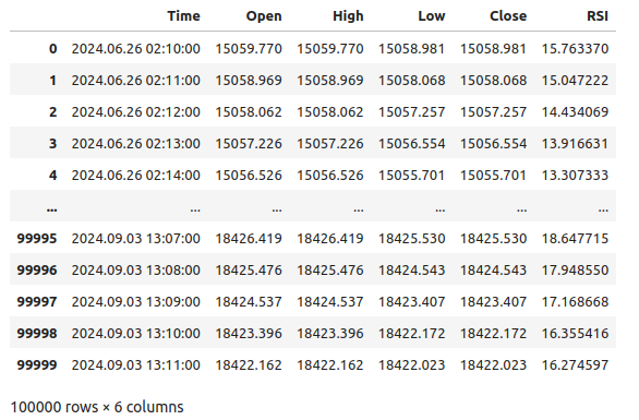
图1：我们的Boom 1000市场数据

现在让我们定义预测范围。

#Define how far into the future we should forecast
look_ahead = 20

现在我们需要定义预测范围，并且为了可视化和绘图目的，还需要向数据中添加附加的标签。

#Let's add targets and labels for plotting
boom_1000["Price Target"] = boom_1000["Close"].shift(-look_ahead)
boom_1000["RSI Target"] = boom_1000["RSI"].shift(-look_ahead)

#Let's also add binary targets for plotting purposes
boom_1000["Price Binary Target"] = np.nan
boom_1000["RSI Binary Target"] = np.nan

#Label the binary targets
boom_1000.loc[boom_1000["Price Target"] < boom_1000["Close"],"Price Binary Target"] = 0
boom_1000.loc[boom_1000["Price Target"] > boom_1000["Close"],"Price Binary Target"] = 1

boom_1000.loc[boom_1000["RSI Target"] < boom_1000["RSI"],"RSI Binary Target"] = 0
boom_1000.loc[boom_1000["RSI Target"] > boom_1000["RSI"],"RSI Binary Target"] = 1

#Drop na values
boom_1000.dropna(inplace=True)

现在让我们定义模型输入和想要比较的两个目标。

#Define the predictors and targets
predictors = ["Open","High","Low","Close","RSI"]
old_target = "Price Binary Target"
new_target = "RSI Binary Target"

探索性数据分析

让我们导入所需的库。

#Exploratory data analysis
import seaborn as sns

显示正在使用的库的版本。

print(f"Seaborn version {sns.__version__}")
Seaborn version 0.13.2

让我们评估由RSI生成的信号的纯度，在我们的理解中，“纯度”回答了这样一个问题：“如果RSI水平下降，价格水平也会下降吗？”我们通过首先统计RSI和价格二进制目标不相等的实例数量，然后将这个数量除以整个数据集中的总行数来计算这个量，最后从1中减去这个比例，得到RSI和价格二进制目标一致的总比例。根据我们的计算，似乎83%的情况下，RSI和价格的变化方向是一致的。

#Let's assess the purity of the signals generated
rsi_purity = 1 - boom_1000.loc[boom_1000["RSI Binary Target"] != boom_1000["Price Binary Target"]].shape[0] / boom_1000.shape[0]
print(f"Price and the RSI tend to move together {rsi_purity * 100}% of the time")

价格和RSI朝着同一方向变动的比例大约是83.69041189061593%

这个比例相当高，这让我们有了一定的信心，认为在可视化数据时可能会得到较好的分离效果。让我们先创建一个分类图，总结RSI水平下降（第0列）或上升（第1列）的所有实例，分别在x轴上表示，而收盘价在y轴上表示。然后，我们将每个点分别涂成蓝色或橙色，以表示Boom 1000价格水平是上升还是下降。从下面的图表中我们可以看到，第0列主要是蓝色，有一些橙色的点，而第1列则相反。这表明RSI在这里似乎是价格变动的一个很好的分隔器。然而，它并不完美，我们将来可能需要一个附加的指标。

#Let's see this purity level we just calculated
sns.catplot(data=boom_1000,x="RSI Binary Target",y="Close",hue="Price Binary Target")

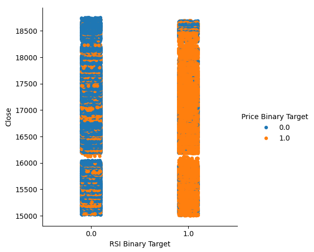
图2：一个分类图，展示我们的RSI如何分割数据

我们还创建了一个散点图，试图可视化RSI与Boom 1000收盘价之间的关系。遗憾的是，正如我们所看到的，两者之间似乎没有任何关系。我们观察到长长的类似意大利面形状的轨迹，蓝色和橙色的点杂乱无章地交替出现，这表明可能还有其他变量影响着目标变量。

#Let us also observe a scatter plot of the two
sns.scatterplot(data=boom_1000,x="RSI",y="Close",hue="Price Binary Target")

图3：RSI读数与收盘价的散点图

也许我们试图可视化的这种关系在二维空间中无法看到，让我们尝试在三维空间中可视化数据，希望我们能够观察到之前未能看到的隐藏的交互效应。

导入我们需要的库。

#Let's create 3D scatter plots
import matplotlib.pyplot as plt

定义要绘制的数据量。

#Define the plot end
end = 10000

现在创建三维散点图。遗憾的是，我们仍然可以观察到数据似乎随机分布，没有任何我们可以利用的明显模式。

#Visualizing our data in 3D
fig = plt.figure(figsize=(7,7))
ax = fig.add_subplot(111,projection='3d')
colors = ['blue' if movement == 0 else 'red' for movement in boom_1000.loc[0:end,"Price Binary Target"]]
ax.scatter(boom_1000.loc[0:end,"RSI"],boom_1000.loc[0:end,"High"],boom_1000.loc[0:end,"Close"],c=colors)

ax.set_xlabel('Boom 1000 RSI')
ax.set_ylabel('Boom 1000 High')
ax.set_zlabel('Boom 1000 Close')

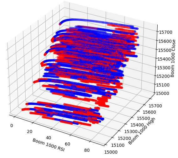
图4：Boom 1000市场及其与RSI关系的三维散点图

现在让我们分析RSI与价格数据之间的相关性水平。我们观察到相关性水平相当低，几乎为0。

#Let's analyze the correlation levels
sns.heatmap(boom_1000.loc[:,predictors].corr(),annot=True)

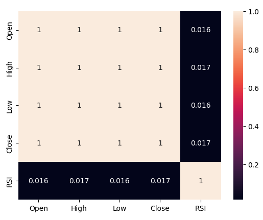
图5：相关矩阵的热力图

准备建模数据

在我们开始建模数据之前，我们首先需要对数据进行缩放和标准化。让我们开始导入需要的库。

#Preparing to model the data
import sklearn
from sklearn.preprocessing import RobustScaler
from sklearn.neural_network import MLPClassifier,MLPRegressor
from sklearn.model_selection import TimeSeriesSplit, train_test_split
from sklearn.metrics import accuracy_score

显示库的版本。

#Display library version
print(f"Sklearn version {sklearn.__version__}")

Sklearn 1.4.1.post1版

缩放数据。

#Scale our data
X = pd.DataFrame(RobustScaler().fit_transform(boom_1000.loc[:,predictors]),columns=predictors)

定义我们的新旧目标。

#Our old and new target
old_y = boom_1000.loc[:,"Price Binary Target"]
new_y = boom_1000.loc[:,"RSI Binary Target"]

执行训练集和测试集的划分。

#Perform train test splits
train_X,test_X,ohlc_train_y,ohlc_test_y = train_test_split(X,old_y,shuffle=False,test_size=0.5)
_,_,rsi_train_y,rsi_test_y = train_test_split(X,new_y,shuffle=False,test_size=0.5)

准备一个数据帧来存储我们在验证中的准确率水平。

#Prepare data frames to store our accuracy levels
validation_accuracy = pd.DataFrame(index=np.arange(0,5),columns=["Close Accuracy","RSI Accuracy"])

现在让我们创建一个时间序列分割对象。

#Let's create the time series split object
tscv =  TimeSeriesSplit(gap=look_ahead,n_splits=5)

数据建模

我们现在准备进行交叉验证，以观察两个可能的目标之间准确率的变化。

#Instatiate the model
model = MLPClassifier(hidden_layer_sizes=(30,10),max_iter=200)
#Cross validate the model
for i,(train,test) in enumerate(tscv.split(train_X)):
        model.fit(train_X.loc[train[0]:train[-1],:],ohlc_train_y.loc[train[0]:train[-1]])
        validation_accuracy.iloc[i,0] = accuracy_score(ohlc_train_y.loc[test[0]:test[-1]],model.predict(train_X.loc[test[0]:test[-1],:]))

我们的准确率水平

validation_accuracy

近似准确率	RSI准确率
0.53703	0.663186
0.544592	0.623575
0.479534	0.597647
0.57064	0.651422
0.545913	0.616373

我们的平均准确率水平可以直观地表明，我们可能更适合预测RSI值的变化。

validation_accuracy.mean()

近似准确率 0.535542
RSI准确率 0.630441
数据类型：对象

标准差越低，模型对其预测的信心就越高。该模型似乎学会了更有把握地预测RSI，而不只是预测价格的变化。

validation_accuracy.std()

近似准确率 0.033765
RSI准确率 0.026613
数据类型：对象

让我们绘制每个模型的性能。

validation_accuracy.plot()

图6：可视化我们的验证准确率

最后，箱线图帮助我们观察两个模型之间的性能差异。正如我们所见，RSI模型的表现远远超过了价格模型。

#Our RSI validation accuracy is better
sns.boxplot(validation_accuracy)

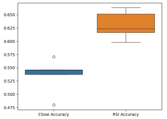
图7：验证中的准确率箱线图

特征的重要性

现在让我们分析哪些特征对预测RSI值很重要，我们将从对神经网络进行的逐步选择开始。逐步选择从一个空模型开始，每次依次添加一个特征，直到无法进一步提升模型的性能为止。

首先，我们导入所需的库。

#Feature importance
import mlxtend
from mlxtend.feature_selection import SequentialFeatureSelector as SFS

现在显示库版本。

print(f"Mlxtend version: {mlxtend.__version__}")

Mlxtend版本：0.23.1

重新初始化模型。

#Reinitialize the model
model = MLPClassifier(hidden_layer_sizes=(30,10),max_iter=200)

设置功能选择器。

#Define the forward feature selector
sfs1 = SFS(
        model,
        k_features=(1,X.shape[1]),
        n_jobs=-1,
        forward=True,
        cv=5,
        scoring="accuracy"
)

安装功能选择器。

#Fit the feature selector
sfs = sfs1.fit(train_X,rsi_train_y)

让我们看看已经识别出的最重要的特征。所有可用的特征都被选中了。

sfs.k_feature_names_

('Open', 'High', 'Low', 'Close', 'RSI')

让我们可视化特征选择过程。首先，我们导入所需的库。

#Importing the libraries we need
from mlxtend.plotting import plot_sequential_feature_selection as plot_sfs
import matplotlib.pyplot as plt

现在我们绘制结果。

fig1 = plot_sfs(sfs.get_metric_dict(), kind='std_err')

plt.title('Sequential Forward Selection')
plt.grid()
plt.show()

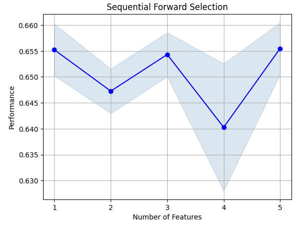
图8：可视化特征选择过程

互信息（Mutual Information，MI）使我们能够了解每个预测因子的潜在价值。MI分数越高，通常该预测因子可能越有价值。MI能够捕捉数据中的非线性依赖关系。最后，MI采用对数尺度，这意味着在实践中，MI分数超过3的情况较为罕见。

导入我们需要的库。

#Let's analyze our MI scores
from sklearn.feature_selection import mutual_info_classif

计算MI分数

mi_scores = pd.DataFrame(mutual_info_classif(train_X,rsi_train_y).reshape(1,5),columns=predictors)

绘制结果表明，根据MI分数，RSI列是最重要的列。

#Let's visualize the results
mi_scores.plot.bar()

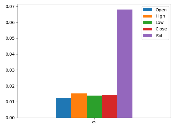
图9：可视化我们的MI分数

参数调整

我们现在将尝试调整模型，以增加更多的性能。Sklearn库中的RandomizedSearchCV模块允许我们轻松地调整机器学习模型。在调整机器学习模型时，需要在准确率与计算时间之间做出权衡。我们通过调整总迭代次数来决定这两者之间的平衡。让我们导入所需的库。

#Parameter tuning
from sklearn.model_selection import RandomizedSearchCV

初始化模型。

#Reinitialize the model
model = MLPClassifier(hidden_layer_sizes=(30,10),max_iter=200)

定义调优器对象。

#Define the tuner
tuner = RandomizedSearchCV(
        model,
        {
                "activation":["relu","tanh","logistic","identity"],
                "solver":["adam","sgd","lbfgs"],
                "alpha":[0.1,0.01,0.001,0.00001,0.000001],
                "learning_rate": ["constant","invscaling","adaptive"],
                "learning_rate_init":[0.1,0.01,0.001,0.0001,0.000001,0.0000001],
                "power_t":[0.1,0.5,0.9,0.01,0.001,0.0001],
                "shuffle":[True,False],
                "tol":[0.1,0.01,0.001,0.0001,0.00001],
        },
        n_iter=300,
        cv=5,
        n_jobs=-1,
        scoring="accuracy"
)

拟合调优器对象。

#Fit the tuner
tuner_results =tuner.fit(train_X,rsi_train_y)

我们已获取的最佳参数。

#Best parameters
tuner_results.best_params_

{'tol': 1e-05,
 'solver': 'lbfgs',
 'shuffle': True,
 'power_t': 0.0001,
 'learning_rate_init': 0.01,
 'learning_rate': 'adaptive',
 'alpha': 1e-06,
 'activation': 'logistic'}

检测过拟合

为了测试是否存在过拟合，我们将在验证数据上对默认模型和定制的模型进行交叉验证。如果默认模型表现更好，那么我们就知道对训练集进行了过拟合。否则，我们就成功地进行了超参数调整。

初始化两个模型。

#Testing for overfitting
default_model = MLPClassifier(hidden_layer_sizes=(30,10),max_iter=200)
customized_model = MLPClassifier(
                                hidden_layer_sizes=(30,10),
                                max_iter=200,
                                tol=0.00001,
                                solver="lbfgs",
                                shuffle=True,
                                power_t=0.0001,
                                learning_rate_init=0.01,
                                learning_rate="adaptive",
                                alpha=0.000001,
                                activation="logistic"
                                )

在训练数据上拟合这两个模型。

#First we will train both models on the training set
default_model.fit(train_X,rsi_train_y)
customized_model.fit(train_X,rsi_train_y)

重置两个数据集的索引。

#Now we will reset our indexes
rsi_test_y = rsi_test_y.reset_index()
test_X = test_X.reset_index()

格式化数据。

#Format the data
rsi_test_y = rsi_test_y.loc[:,"RSI Binary Target"]
test_X = test_X.loc[:,predictors]

准备一个数据帧来存储我们的准确率。

#Prepare a data frame to store our accuracy levels
validation_error = pd.DataFrame(index=np.arange(0,5),columns=["Default Neural Network","Customized Neural Network"])

交叉验证每个模型以测试过拟合。

#Perform cross validation
for i,(train,test) in enumerate(tscv.split(test_X)):
        customized_model.fit(test_X.loc[train[0]:train[-1],predictors],rsi_test_y.loc[train[0]:train[-1]])
        validation_error.iloc[i,1] = accuracy_score(rsi_test_y.loc[test[0]:test[-1]],customized_model.predict(test_X.loc[test[0]:test[-1]]))

我们验证中的性能水平。

validation_error

默认神经网络	定制神经网络
0.627656	0.597767
0.637258	0.635938
0.621414	0.631977
0.6429	0.6411
0.664866	0.652503

通过分析我们的平均表现水平可以清楚地表明，默认模型比定制模型略胜一筹。

validation_error.mean()

默认神经网络 0.638819
定制神经网络 0.631857
数据类型：对象

此外，我们的定制模型由于其准确率得分的方差更低，表现出了更高的技能水平。

validation_error.std()

默认神经网络 0.016771
定制神经网络 0.020557
数据类型：对象

让我们绘制结果。

validation_error.plot()

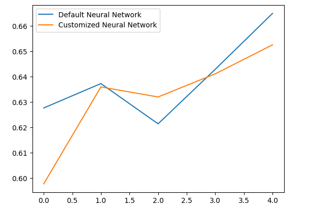
图10：可视化我们的过拟合测试

箱线图显示，我们的定制模型似乎不够稳定，它存在一些默认模型中未观察到的异常值。此外，默认模型平均表现略好一些。因此，我们将选择默认模型而不是定制模型。

sns.boxplot(validation_error)

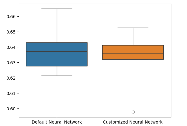
图11：可视化我们的过拟合测试 II

准备导出为ONNX格式

在将模型导出为ONNX格式之前，我们必须首先以一种可以在MetaTrader 5终端中复现的方式对数据进行缩放。我们将从每一列中减去该列的均值，并除以该列的标准差，这样操作可确保在数据范围不同的情况下，模型能够有效地学习。此外，我们还将以CSV格式导出均值和标准差的值，以便供我们后续检索。

#Preparing to export to ONNX
#Let's scale our data
scaling_factors = pd.DataFrame(columns=predictors,index=['mean','standard deviation'])
X = boom_1000.loc[:,predictors]
y = boom_1000.loc[:,"RSI Target"]

缩放每列。

#Let's fill each column
for i in np.arange(0,len(predictors)):
        scaling_factors.iloc[0,i] = X.iloc[:,i].mean()
        scaling_factors.iloc[1,i] = X.iloc[:,i].std()
        X.iloc[:,i] = ( ( X.iloc[:,i] - scaling_factors.iloc[0,i] ) / scaling_factors.iloc[1,i])

以CSV格式保存缩放因子。

#Save the scaling factors as a CSV
scaling_factors.to_csv("/home/volatily/.wine/drive_c/Program Files/MetaTrader 5/MQL5/Files/boom_1000_scaling_factors.csv")

导出到ONNX

开放神经网络交换（ONNX） 是一个开源的可互操作的机器学习框架，它允许开发人员在支持ONNX API的任何编程语言中构建、共享和使用机器学习模型。这使得我们能够使用Python构建机器学习模型，并在生产环境中以MQL5进行部署。

首先，我们导入所需的库。

#Exporting to ONNX
import onnx
import netron
import skl2onnx
from skl2onnx import convert_sklearn
from skl2onnx.common.data_types import FloatTensorType

显示库的版本。

#Display the library versions
print(f"Onnx version {onnx.__version__}")
print(f"Netron version {netron.__version__}")
print(f"Skl2onnx version {skl2onnx.__version__}")

Onnx 版本 1.15.0
Netron 版本 7.8.0
Skl2onnx版本 1.16.0

定义模型的输入类型。

#Define the model input types
initial_types = [("float_input",FloatTensorType([1,5]))]

基于我们现有的全部数据拟合模型。

#Fit the model on all the data we have
default_model = MLPRegressor(hidden_layer_sizes=(30,10),max_iter=200)
default_model.fit(X,y)

将模型转换为ONNX的表示形式。

#Convert the model to an ONNX representation
onnx_model = convert_sklearn(default_model,initial_types=initial_types,target_opset=12)

将ONNX的表示形式保存为文件。

#Save the ONNX representation
onnx_name = "Boom 1000 Neural Network.onnx"
onnx.save(onnx_model,onnx_name)

使用netron查看模型。

#View the onnx model
netron.start(onnx_name)

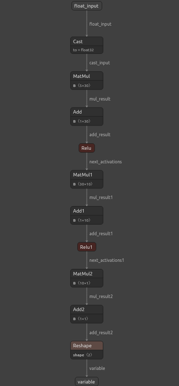
图12：可视化我们的深度神经网络

图13：可视化我们模型的输入和输出

在MQL5中的实现

为了构建一个集成人工智能系统的交易应用程序，我们首先需要用到刚才在Python中导出的ONNX模型。

//+------------------------------------------------------------------+
//|                                                    Boom 1000.mq5 |
//|                                        Gamuchirai Zororo Ndawana |
//|                          https://www.mql5.com/en/gamuchiraindawa |
//+------------------------------------------------------------------+
#property copyright "Gamuchirai Zororo Ndawana"
#property link      "https://www.mql5.com/en/gamuchiraindawa"
#property version   "1.00"

//+------------------------------------------------------------------+
//| ONNX Model                                                       |
//+------------------------------------------------------------------+
#resource "\\Files\\Boom 1000 Neural Network.onnx" as const uchar onnx_buffer[];

让我们同时加载交易库，以便管理我们的仓位。

//+-----------------------------------------------------------------+
//| Libraries we need                                               |
//+-----------------------------------------------------------------+
#include <Trade/Trade.mqh>
CTrade Trade;

定义我们将在整个程序中使用的全局变量。

//+------------------------------------------------------------------+
//| Global variables                                                 |
//+------------------------------------------------------------------+
long onnx_model;
int rsi_handler,model_state,system_state;
double mean_values[5],std_values[5],rsi_buffer[],bid,ask;
vectorf model_outputs = vectorf::Zeros(1);
vectorf model_inputs = vectorf::Zeros(5);

现在让我们定义一个用于准备ONNX模型的函数。该函数将首先从我们在程序开头定义的缓冲区中创建模型，并验证该模型是否损坏。如果模型损坏，函数将返回false，这样会终止初始化过程。从此，该函数将继续设置ONNX模型的输入和输出形状。如果我们未能定义输入或输出参数中的任何一个，函数将再次返回false并终止初始化过程。

//+------------------------------------------------------------------+
//| This function will prepare our ONNX model                        |
//+------------------------------------------------------------------+
bool load_onnx_model(void)
  {
//--- First create the ONNX model from the buffer we created earlier
   onnx_model = OnnxCreateFromBuffer(onnx_buffer,ONNX_DEFAULT);

//--- Validate the ONNX model
   if(onnx_model == INVALID_HANDLE)
     {
      Comment("[ERROR] Failed to create the ONNX model: ",GetLastError());
      return(false);
     }

//--- Set the input and output shapes of the model
   ulong input_shape[] = {1,5};
   ulong output_shape[] = {1,1};

//--- Validate the input and output shape
   if(!OnnxSetInputShape(onnx_model,0,input_shape))
     {
      Comment("Failed to set the ONNX model input shape: ",GetLastError());
      return(false);
     }

   if(!OnnxSetOutputShape(onnx_model,0,output_shape))
     {
      Comment("Failed to set the ONNX model output shape: ",GetLastError());
      return(false);
     }

   return(true);
  }

如果没有对模型输入进行缩放，我们将无法使用ONNX模型。以下函数将把我们需要的均值和标准差加载到可以轻松访问的数组中。

//+-----------------------------------------------------------------+
//| Load the scaling values                                         |
//+-----------------------------------------------------------------+
void load_scaling_values(void)
  {
//--- BOOM 1000 OHLC + RSI Mean values
   mean_values[0] = 16799.87389394667;
   mean_values[1] = 16800.872890865994;
   mean_values[2] = 16798.91007345616;
   mean_values[3] = 16799.908906749482;
   mean_values[4] = 43.45867626462568;
//--- BOOM 1000 OHLC + RSI Mean std values
   std_values[0] = 864.3356132780019;
   std_values[1] = 864.3839684000297;
   std_values[2] = 864.2859346216392;
   std_values[3] = 864.3344430387272;
   std_values[4] = 20.593175501388043;
  }
//+------------------------------------------------------------------+

我们还需要定义一个函数，用于获取最新的市场价格以及当前的技术指标值。

//+------------------------------------------------------------------+
//| Fetch updated market prices and technical indicator values       |
//+------------------------------------------------------------------+
void update_market_data(void)
  {
//--- Market data
   bid = SymbolInfoDouble(Symbol(),SYMBOL_BID);
   ask = SymbolInfoDouble(Symbol(),SYMBOL_ASK);
//--- Technical indicator values
   CopyBuffer(rsi_handler,0,0,1,rsi_buffer);
  }

最后，我们需要一个函数来获取模型的输入，对它们进行缩放，并从模型中获取预测结果。我们将保留一个标识来记住模型的预测结果，这将帮助我们轻松地找出到模型何时能够预测到反转。

//+------------------------------------------------------------------+
//| Fetch a prediction from our model                                |
//+------------------------------------------------------------------+
void model_predict(void)
  {
//--- Get the model inputs
   model_inputs[0] = iOpen(_Symbol,PERIOD_CURRENT,0);
   model_inputs[1] = iHigh(_Symbol,PERIOD_CURRENT,0);
   model_inputs[2] = iLow(_Symbol,PERIOD_CURRENT,0);
   model_inputs[3] = iClose(_Symbol,PERIOD_CURRENT,0);
   model_inputs[4] = rsi_buffer[0];

//--- Scale the model inputs
   for(int i = 0; i < 5; i++)
     {
      model_inputs[i] = ((model_inputs[i] - mean_values[i]) / std_values[i]);
     }

//--- Fetch a prediction from our model
   OnnxRun(onnx_model,ONNX_DEFAULT,model_inputs,model_outputs);
//--- Give user feedback
   Comment("Model RSI Forecast: ",model_outputs[0]);
//--- Store the model's state
   if(rsi_buffer[0] > model_outputs[0])
     {
      model_state = -1;
     }

   else
      if(rsi_buffer[0] < model_outputs[0])
        {
         model_state = 1;
        }
  }

现在，我们将定义模型的初始化过程。我们首先会加载ONNX模型，然后获取缩放值并设置相对强弱指标（RSI）。

//+------------------------------------------------------------------+
//| Expert initialization function                                   |
//+------------------------------------------------------------------+
int OnInit()
  {
//--- This function will prepare our ONNX model and set the input and output shapes
   if(!load_onnx_model())
     {
      return(INIT_FAILED);
     }

//--- This function will prepare our scaling values
   load_scaling_values();

//--- Setup our technical indicatot
   rsi_handler = iRSI(Symbol(),PERIOD_CURRENT,20,PRICE_CLOSE);

//--- Everything went fine
   return(INIT_SUCCEEDED);
  }

每当应用程序从图表中移除时，我们将释放不再使用的资源，包括释放ONNX模型、RSI指标并移除EA。

//+------------------------------------------------------------------+
//| Expert deinitialization function                                 |
//+------------------------------------------------------------------+
void OnDeinit(const int reason)
  {
//--- Release the resources we no longer need
   OnnxRelease(onnx_model);
   IndicatorRelease(rsi_handler);
   ExpertRemove();
  }

每当接收到更新的价格时，我们首先会获取最新的市场和技术数据，这包括买入价和卖出价以及RSI的读数。然后我们就可以准备从模型中获取新的预测了。如果没有开仓，我们将按照模型的预测进行操作，并使用一个二进制标识来记住我们当前的仓位情况。否则，如果我们已经有一个仓位，我们将检查模型的新预测是否与我们的开仓方向相反。如果是，我们将平仓。否则，我们将继续获利。

//+------------------------------------------------------------------+
//| Expert tick function                                             |
//+------------------------------------------------------------------+
void OnTick()
  {
//--- Fetch updated market prices
   update_market_data();

//--- On every tick we need to fetch a prediction from our model
   model_predict();

//--- If we have no open positions, follow the model's prediction
   if(PositionsTotal() == 0)
     {
      //--- Our model detected a spike
      if(model_state == 1)
        {
         Trade.Buy(0.2,Symbol(),ask,0,0,"BOOM 1000 AI");
         system_state = 1;
        }

      //--- Our model detected a drop
      if(model_state == -1)
        {
         Trade.Sell(0.2,Symbol(),bid,0,0,"BOOM 1000 AI");
         system_state = -1;
        }
     }

//--- If we have open positiosn, our AI system will decide when to close them
   else
      if(PositionsTotal() > 0)
        {
         if(system_state != model_state)
           {
            //--- Close the positions we opened
            Alert("Reversal detected by the AI system,closing all positions now!");
            Trade.PositionClose(Symbol());
           }
        }
  }
//+------------------------------------------------------------------+

图14：我们的Boom 1000系统成功捕捉到了一次价格飙升

图15：我们的Boom 1000系统检测到了一次反转

结论

在今天的文章中，我们已经证明可以构建能够自优化的EA来应对最具挑战性的合成工具，此外，还可以表明，直接预测价格水平的传统方法已经不足以适应当今的算法市场。