
重构经典策略(第十部分):人工智能(AI)能否为MACD提供动力?

移动平均线交叉可能是现存最古老的交易策略之一。平滑异同移动平均线(MACD)是一个非常流行的指标,它是基于移动平均线交叉的概念构建的。我们社区中可能有许多新成员,也许对MACD指标的预测能力感到好奇,因为他们正在寻找构建最优交易策略的方法。此外,还有一些经验丰富的技术分析师在策略中使用MACD,他们可能也有同样的疑问。本文将为您提供关于MACD指标在欧元兑美元货币对上预测能力的实证分析。此外,我们还将为您提供一些建模技术,您可以利用这些技术结合AI来强化技术分析。
交易策略概述
MACD指标主要用于识别市场趋势并衡量趋势动能。该指标由已故的杰拉尔德·阿佩尔(Gerrald Appel)于20世纪70年代创立。阿佩尔曾为其私人客户担任资金经理,他的成功源于其基于技术分析的交易方法。他在大约50年前发明了MACD指标。

图1:MACD指标的创造者杰拉尔德·阿佩尔
技术分析师以各种方式使用该指标来确定入场和离场点。下图2是将MACD指标应用于英镑兑美元(GBPUSD)货币对的截图,使用其默认设置。该指标默认包含在您的MetaTrader 5安装中。红色线条,称为MACD主线,是通过计算两个移动平均线之间的差值得出的,一个较快,另一个较慢。每当主线穿过0以下时,市场很可能处于下跌趋势,而当该线穿过0以上时,情况则相反。
同样,主线本身也可以用来判断市场强度。只有价格上涨时,主线的值才会增加,而价格下跌时,主线则会下降。因此,主线形成类似杯子形状的转折点是由市场动能的转变造成的。围绕MACD已经实施了各种交易策略。更复杂和精细的策略试图识别MACD背离。
MACD背离发生在价格水平在一个强劲趋势中上涨,突破新的极端水平时。而另一方面,MACD指标处于一个趋势中,该趋势仅逐渐变浅,并开始下跌,与图表上看到的强劲价格走势形成鲜明的对比。通常,MACD背离被解释为趋势反转的早期预警,允许交易者在市场变得更加动荡之前平仓。
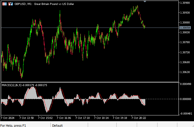
图2:在英镑兑美元M1图表上使用默认设置的MACD指标
有许多怀疑论者质疑MACD指标的使用。让我们先解决一个显而易见的问题。所有技术指标都被归类为滞后指标。这意味着,技术指标只有在价格水平发生变化后才会改变,它们不能在价格水平变化之前改变。像全球通货膨胀水平这样的宏观经济指标和像战争爆发或自然灾害这样的地缘政治新闻,可能会抵消供求水平。它们被认为是领先指标,因为它们可以在价格水平反映变化之前迅速改变。
许多交易者认为,这些滞后信号很可能会导致交易者在市场走势已经耗尽时才开仓。此外,观察到趋势反转并没有MACD背离作为先兆的情况也很常见。同样,也有可能观察到MACD背离并没有导致趋势反转。
这些事实促使我们质疑该指标的可靠性,以及它是否真的具有值得信赖的预测能力。我们希望评估是否可以使用AI克服该指标固有的滞后性。如果MACD指标被证明是可靠的,我们将整合一个人工智能模型,该模型可以:
- 使用指标值来预测未来的价格水平。
- 预测MACD指标本身。
具体取决于哪种建模方法产生的误差更低。否则,如果我们的分析表明,在我们当前的策略下,MACD可能没有预测能力,那么我们将选择在预测价格水平时表现最优的模型。
方法论概述
我们的分析始于用MQL5编写的定制脚本,该脚本从欧元兑美元的M1市场报价中精确地获取了100,000行数据,以及它们对应的MACD信号和主值,并将这些数据保存到一个CSV文件中。根据我们的数据可视化结果,MACD指标似乎是一个对未来价格水平区分能力较差的指标。价格水平的变化很可能与指标值无关,此外,指标的计算还赋予了数据一种非线性和复杂的结构,可能导致建模困难。
从我们的MetaTrader 5终端获得的数据被分成了两部分。我们使用第一部分通过5折交叉验证来估计我们模型的准确性。随后,我们创建了三个相同的深度神经网络(Deep Neural Network)模型,并在数据的三个不同子集上训练它们:
- 价格模型:使用MetaTrader 5的OHLC市场报价来预测价格水平。
- MACD模型:使用OHLC报价和MACD读数来预测MACD指标值。
- 完整模型:使用OHLC报价和MACD指标来预测价格水平。
数据集的后半部分用于测试这些模型。第一个模型在测试中得分最高,准确率为69%。我们的特征选择算法表明,我们从MetaTrader 5获得的市场报价比MACD值更有信息量。
因此,我们开始优化现有的最优模型,这是一个预测欧元兑美元未来价格的回归模型。然而,我们很快遇到了问题,因为我们的模型学习了训练数据中的噪声。我们在测试集上惨败于一个简单的线性回归。因此,我们将过度优化的模型替换为支持向量机(SVM)。
随后,我们将SVM模型导出为ONNX格式,并使用结合预测未来欧元兑美元价格水平和MACD指标的方法构建了一个EA。
获取我们需要的数据
为了开始我们的工作,我们首先进入MetaEditor集成开发环境(IDE)。我们创建了以下脚本,从MetaTrader 5终端获取市场数据。我们请求了100,000行历史M1数据,并将其导出为CSV格式。以下脚本将用时间、开盘价、最高价、最低价、收盘价以及两个MACD值填充我们的CSV文件。如果您希望跟随我们的步骤,只需将脚本拖放到您想要分析的任何货币对上即可。
//+------------------------------------------------------------------+
//|                                                      ProjectName |
//|                                      Copyright 2020, CompanyName |
//|                                       http://www.companyname.net |
//+------------------------------------------------------------------+
#property copyright "Gamuchirai Zororo Ndawana"
#property link      "https://www.mql5.com/en/users/gamuchiraindawa"
#property version   "1.00"
#property script_show_inputs

//+------------------------------------------------------------------+
//| Script Inputs                                                    |
//+------------------------------------------------------------------+
input int size = 100000; //How much data should we fetch?

//+------------------------------------------------------------------+
//| Global variables                                                 |
//+------------------------------------------------------------------+
int indicator_handler;
double indicator_buffer[];
double indicator_buffer_2[];

//+------------------------------------------------------------------+
//| On start function                                                |
//+------------------------------------------------------------------+
void OnStart()
  {

//--- Load indicator
   indicator_handler = iMACD(Symbol(),PERIOD_CURRENT,12,26,9,PRICE_CLOSE);
   CopyBuffer(indicator_handler,0,0,size,indicator_buffer);
   CopyBuffer(indicator_handler,1,0,size,indicator_buffer_2);
   ArraySetAsSeries(indicator_buffer,true);
   ArraySetAsSeries(indicator_buffer_2,true);

//--- File name
   string file_name = "Market Data " + Symbol() +" MACD " +  ".csv";

//--- Write to file
   int file_handle=FileOpen(file_name,FILE_WRITE|FILE_ANSI|FILE_CSV,",");

   for(int i= size;i>=0;i--)
     {
      if(i == size)
        {
         FileWrite(file_handle,"Time","Open","High","Low","Close","MACD Main","MACD Signal");
        }

      else
        {
         FileWrite(file_handle,iTime(Symbol(),PERIOD_CURRENT,i),
                   iOpen(Symbol(),PERIOD_CURRENT,i),
                   iHigh(Symbol(),PERIOD_CURRENT,i),
                   iLow(Symbol(),PERIOD_CURRENT,i),
                   iClose(Symbol(),PERIOD_CURRENT,i),
                   indicator_buffer[i],
                   indicator_buffer_2[i]
                  );
        }
     }
//--- Close the file
   FileClose(file_handle);
  }
//+------------------------------------------------------------------+
数据预处理
现在已经将数据导出为CSV格式,让我们在Python工作空间中读取这些数据。首先,我们将加载所需的库。
#Load libraries
import pandas as pd
import numpy as np
import seaborn as sns
import matplotlib.pyplot as plt
读取数据。
#Read in the data
data = pd.read_csv("Market Data EURUSD MACD .csv")
定义我们应该对未来多久进行预测。
#Forecast horizon
look_ahead = 20
让我们为欧元兑美元的收盘价和MACD主线添加二进制目标,以标记当前读数是否大于其之前的20个实例。
#Let's add labels
data["Bull Bear"] = np.where(data["Close"] < data["Close"].shift(look_ahead),0,1)
data["MACD Bull"] = np.where(data["MACD Main"] < data["MACD Main"].shift(look_ahead),0,1)

data = data.loc[20:,:]

data
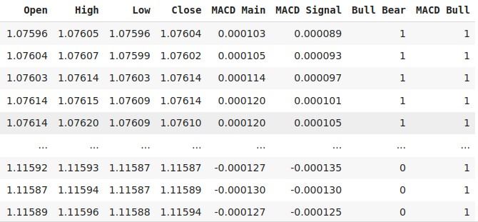
图3:我们数据结构中的部分列
此外,我们还需要定义目标值。
data["MACD Target"] = data["MACD Main"].shift(-look_ahead)
data["Price Target"] = data["Close"].shift(-look_ahead)

data["MACD Binary Target"] = np.where(data["MACD Main"] < data["MACD Target"],1,0)
data["Price Binary Target"] = np.where(data["Close"] < data["Price Target"],1,0)

data = data.iloc[:-20,:]
探索性数据分析
散点图有助于我们可视化因变量和自变量之间的关系。以下图表显示,未来价格水平与当前的MACD读数之间确实存在关系,问题是这种关系是非线性的,并且似乎具有复杂的结构。目前还不清楚MACD指标的变化会引起看涨或看跌的价格表现。
sns.scatterplot(data=data,x="MACD Main",y="MACD Signal",hue="Price Binary Target")
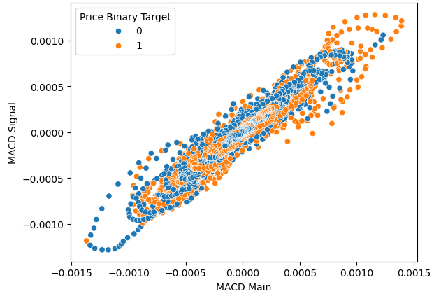
图4:可视化MACD指标与价格水平之间的关系
通过三维绘图进一步证明了这种关系的复杂性。没有明确的边界,因此我们的预期数据将很难分类。我们从图表中唯一能得出的合理推断是,市场在经历MACD的极端水平后,似乎会迅速重新聚集到中心区域。
#Define the 3D Plot
fig = plt.figure(figsize=(7,7))
ax = plt.axes(projection="3d")
ax.scatter(data["MACD Main"],data["MACD Signal"],data["Close"],c=data["Price Binary Target"])
ax.set_xlabel("MACD Main")
ax.set_ylabel("MACD Signal")
ax.set_zlabel("EURUSD Close")
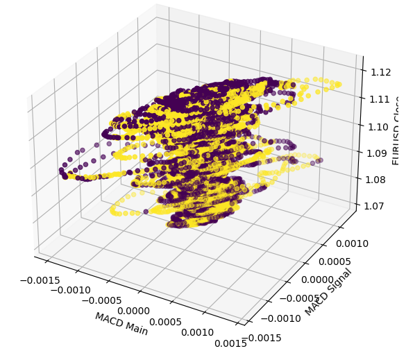
图5:可视化MACD指标与欧元兑美元市场之间的相互作用
小提琴图能让我们在可视化数据分布情况的同时,对两组分布进行比较。图中蓝色轮廓总结了MACD指标上升或下降后,对于未来价格水平的观测分布情况。在接下来的图6中,我们想要探究MACD指标的上升或下降是否与未来价格走势的不同分布存在关联。可以看到,这两组分布几乎一模一样。此外,每组分布的核心位置都有一个箱线图。无论指标处于看涨还是看跌状态,两个箱线图的均值看起来都几乎相同。
sns.violinplot(data=data,x="MACD Bull",y="Close",hue="Price Binary Target",split=True,fill=False)
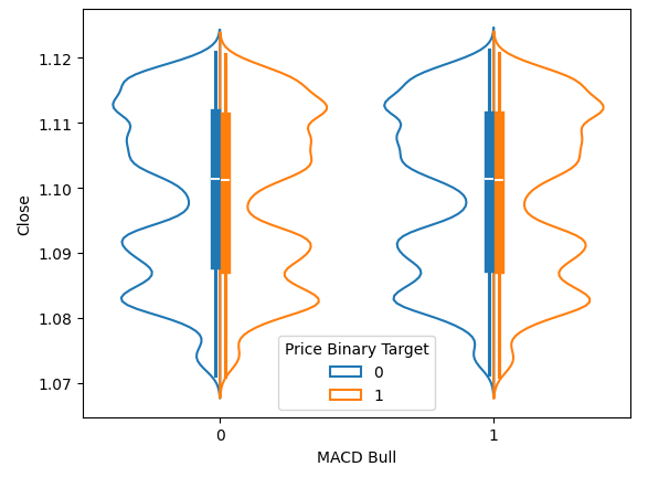
图6:可视化MACD指标对未来价格水平的影响
准备建模数据
现在,我们开始对数据进行建模。首先,导入所需的库。
#Perform train test splits
from sklearn.model_selection import train_test_split,TimeSeriesSplit
from sklearn.metrics import accuracy_score
train,test = train_test_split(data,test_size=0.5,shuffle=False)
现在我们将定义预测器和目标。
#Let's scale the data
ohlc_predictors = ["Open","High","Low","Close","Bull Bear"]
macd_predictors = ["MACD Main","MACD Signal","MACD Bull"]
all_predictors  = ohlc_predictors + macd_predictors
cv_predictors   = [ohlc_predictors,macd_predictors,all_predictors]

#Define the targets
cv_targets = ["MACD Binary Target","Price Binary Target","All"]
缩放数据。
#Scaling the data
from sklearn.preprocessing import MinMaxScaler
scaler = MinMaxScaler()
scaler.fit(train[all_predictors])
train_scaled = pd.DataFrame(scaler.transform(train[all_predictors]),columns=all_predictors)
test_scaled = pd.DataFrame(scaler.transform(test[all_predictors]),columns=all_predictors)
让我们加载所需的库。
#Import the models we will evaluate
from sklearn.neural_network import MLPClassifier,MLPRegressor
from sklearn.linear_model import LinearRegression
创建时间序列拆分对象。
tscv = TimeSeriesSplit(n_splits=5,gap=look_ahead) 我们数据结构的索引将映射到正在评估的输入集。
err_indexes = ["MACD Train","Price Train","All Train","MACD Test","Price Test","All Test"]
现在我们将创建一个数据结构,用于记录在改变输入时对模型准确性的评估。
#Now let us define a table to store our error levels
columns = ["Model Accuracy"]

cv_err = pd.DataFrame(columns=columns,index=err_indexes)
重置所有索引。
#Reset index
train = train.reset_index(drop=True)
test = test.reset_index(drop=True)
让我们对模型进行交叉验证。我们将在训练集上对模型进行交叉验证,然后记录模型在测试集上的准确性,而不会对模型进行拟合。
#Initailize the model
price_model = MLPClassifier(hidden_layer_sizes=(10,6))
macd_model  = MLPClassifier(hidden_layer_sizes=(10,6))
all_model   = MLPClassifier(hidden_layer_sizes=(10,6))

price_acc = []
macd_acc = []
all_acc = []

#Cross validate each model twice
for j,(train_index,test_index) in enumerate(tscv.split(train_scaled)):
  #Fit the models
  price_model.fit(train_scaled.loc[train_index,ohlc_predictors],train.loc[train_index,"Price Binary Target"])
  macd_model.fit(train_scaled.loc[train_index,all_predictors],train.loc[train_index,"MACD Binary Target"])
  all_model.fit(train_scaled.loc[train_index,all_predictors],train.loc[train_index,"Price Binary Target"])
  #Store the accuracy
  price_acc.append(accuracy_score(train.loc[test_index,"Price Binary Target"],price_model.predict(train_scaled.loc[test_index,ohlc_predictors])))
  macd_acc.append(accuracy_score(train.loc[test_index,cv_targets[0]],macd_model.predict(train_scaled.loc[test_index,all_predictors])))
  all_acc.append(accuracy_score(train.loc[test_index,cv_targets[1]],all_model.predict(train_scaled.loc[test_index,all_predictors])))

#Now we can store our estimates of the model's error
cv_err.iloc[0,0] = np.mean(price_acc)
cv_err.iloc[1,0] = np.mean(macd_acc)
cv_err.iloc[2,0] = np.mean(all_acc)
#Estimating test error
cv_err.iloc[3,0] = accuracy_score(test[cv_targets[1]],price_model.predict(test_scaled[ohlc_predictors]))
cv_err.iloc[4,0] = accuracy_score(test[cv_targets[0]],macd_model.predict(test_scaled[all_predictors]))
cv_err.iloc[5,0] = accuracy_score(test[cv_targets[1]],all_model.predict(test_scaled[all_predictors]))
| 输入组 | 模型准确性 |
|---|---|
| MACD训练 | 0.507129 |
| OHLC训练 | 0.690267 |
| 所有训练 | 0.504577 |
| MACD测试 | 0.48669 |
| OHLC测试 | 0.684069 |
| 所有测试 | 0.487442 |
特征的重要性
现在让我们尝试评估深度神经网络的特征重要性水平。我们将选择排列重要性来解释模型。排列重要性通过首先打乱输入列的值,然后评估模型准确性的变化,来定义每个输入特征的重要性。其想法是,重要的特征会引起误差大幅下降,而不重要的特征会导致模型准确性的变化接近于0。
然而,有一些需要考虑的因素。首先,排列重要性算法会随机打乱模型的每个输入。这意味着该算法可能会随机打乱开盘价,并将其设置得高于最高价。这在现实世界中显然是不可能的。因此,我们应该谨慎地解释该算法的结果。有人可能会说该算法存在偏差,因为它在可能永远不会发生的模拟条件下评估特征的重要性,从而让模型遭到非必要地惩罚。此外,由于用于拟合现代神经网络优化算法的随机性,使用相同的数据集训练相同的神经网络可能会得到截然不同的解释。
#Let us try assess feature importance
from sklearn.inspection import permutation_importance
from sklearn.linear_model import RidgeClassifier
现在我们将对训练好的深度神经网络模型拟合排列重要性对象。您可以选择传递训练数据或测试数据以进行打乱,我们选择了测试数据。之后,我们按照导致准确性下降的顺序排列数据,并绘制了结果。下图7显示了观察到的排列重要性分数。我们可以看到,与MACD相关的输入被打乱后的影响非常接近于0,这意味着MACD列对模型并不重要。
#Let us fit the model
model   = MLPClassifier(hidden_layer_sizes=(10,6))
model.fit(train_scaled.loc[:,all_predictors],train.loc[:,"Price Binary Target"])

#Calculate permutation importance scores
pi = permutation_importance(
    model, test_scaled.loc[:,all_predictors], test.loc[:,"Price Binary Target"], n_repeats=10, random_state=42, n_jobs=-1
)

#Sort the importance scores
sorted_importances_idx = pi.importances_mean.argsort()
importances = pd.DataFrame(
    pi.importances[sorted_importances_idx].T,
    columns=test_scaled.columns[sorted_importances_idx],
)

#Create the plot
ax = importances.plot.box(vert=False, whis=10)
ax.set_title("Permutation Importances (test set)")
ax.axvline(x=0, color="k", linestyle="--")
ax.set_xlabel("Decrease in accuracy score")
ax.figure.tight_layout()
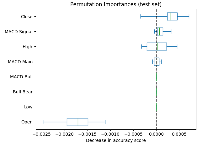
图7:我们的排列重要性分数将收盘价列为最重要的特征
拟合一个更简单的模型也可以让我们了解输入的重要性水平。岭分类器是一个线性模型,它将系数推向越来越接近0的方向,以最小化其误差。因此,假设您的数据已经被标准化和缩放,不重要的特征将具有最小的岭系数。如果您感到好奇的话,岭分类器可以通过将普通线性模型扩展为包括一个与模型系数平方和成比例的惩罚项来实现这一点。这通常被称为L2正则化。
#Let us fit the model
model   = RidgeClassifier()
model.fit(train_scaled.loc[:,all_predictors],train.loc[:,"Price Binary Target"])
现在让我们绘制模型的系数。
ridge_importance = pd.DataFrame(model.coef_.tolist(),columns=all_predictors)

#Prepare the plot
fig,ax = plt.subplots(figsize=(10,5))
sns.barplot(ridge_importance,ax=ax)
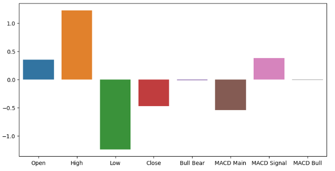
图8:我们的岭系数表明,最高价和最低价是拥有的最有信息量的特征
参数调整
现在我们将尝试优化表现最佳的模型。然而正如之前提到的,我们的优化程序这次并不成功。遗憾的是,这是优化算法的固有特性,我们不能保证能找到解决方案。执行参数优化并不一定意味着最终得到的模型会更好,我们只是试图近似最优模型参数。让我们加载所需的库。
#Let's tune our model further
from sklearn.model_selection import RandomizedSearchCV
定义模型。
#Reinitialize the model
model  = MLPRegressor(max_iter=200)
现在我们将定义调优器对象。该对象将在不同的初始化参数下评估我们的模型,并返回一个包含找到的最优输入的对象。
#Define the tuner
tuner = RandomizedSearchCV(
        model,
        {
        "activation" : ["relu","logistic","tanh","identity"],
        "solver":["adam","sgd","lbfgs"],
        "alpha":[0.1,0.01,0.001,0.0001,0.00001,0.00001,0.0000001],
        "tol":[0.1,0.01,0.001,0.0001,0.00001,0.000001,0.0000001],
        "learning_rate":['constant','adaptive','invscaling'],
        "learning_rate_init":[0.1,0.01,0.001,0.0001,0.00001,0.000001,0.0000001],
        "hidden_layer_sizes":[(2,4,8,2),(10,20),(5,10),(2,20),(6,8,10),(1,5),(20,10),(8,4),(2,4,8),(10,5)],
        "early_stopping":[True,False],
        "warm_start":[True,False],
        "shuffle": [True,False]
        },
        n_iter=100,
        cv=5,
        n_jobs=-1,
        scoring="neg_mean_squared_error"
)
拟合调优器对象。
tuner.fit(train.loc[:,ohlc_predictors],train.loc[:,"Price Target"]) 我们找到的最优参数。
tuner.best_params_
'tol': 0.01,
'solver': 'sgd',
'shuffle': False,
'learning_rate_init': 0.01,
'learning_rate': 'constant',
'hidden_layer_sizes': (20, 10),
'early_stopping': True,
'alpha': 1e-07,
'activation': 'identity'}
深度优化
可以通过使用SciPy库来更深入地寻找更好的输入设置。我们将利用该库对模型的连续参数进行全局优化的结果进行估计。#Deeper optimization from scipy.optimize import minimize from sklearn.metrics import mean_squared_error from sklearn.model_selection import TimeSeriesSplit
定义一个时间序列分割对象。
#Define the time series split object
tscv = TimeSeriesSplit(n_splits=5,gap=look_ahead)
创建数据结构以存储我们的准确性水平。
#Create a dataframe to store our accuracy
current_error_rate = pd.DataFrame(index = np.arange(0,5),columns=["Current Error"])
algorithm_progress = []
我们要最小化的目标函数将是模型在训练数据上的误差水平。
#Define the objective function
def objective(x):
    #The parameter x represents a new value for our neural network's settings
    model = MLPRegressor(hidden_layer_sizes=tuner.best_params_["hidden_layer_sizes"],
                         early_stopping=tuner.best_params_["early_stopping"],
                         warm_start=tuner.best_params_["warm_start"],
                         max_iter=500,
                         activation=tuner.best_params_["activation"],
                         learning_rate=tuner.best_params_["learning_rate"],
                         solver=tuner.best_params_["solver"],
                         shuffle=tuner.best_params_["shuffle"],
                         alpha=x[0],
                         tol=x[1],
                         learning_rate_init=x[2]
                         )
    #Now we will cross validate the model
    for i,(train_index,test_index) in enumerate(tscv.split(train)):
        #Train the model
        model.fit(train.loc[train_index,ohlc_predictors],train.loc[train_index,"Price Target"])
        #Measure the RMSE
        current_error_rate.iloc[i,0] = mean_squared_error(train.loc[test_index,"Price Target"],model.predict(train.loc[test_index,ohlc_predictors]))
    #Store the algorithm's progress
    algorithm_progress.append(current_error_rate.iloc[:,0].mean())
    #Return the Mean CV RMSE
    return(current_error_rate.iloc[:,0].mean())
SciPy希望我们提供初始值以启动优化程序。
#Define the starting point
pt = [tuner.best_params_["alpha"],tuner.best_params_["tol"],tuner.best_params_["learning_rate_init"]]
bnds = ((10.00 ** -100,10.00 ** 100),
        (10.00 ** -100,10.00 ** 100),
        (10.00 ** -100,10.00 ** 100))
现在让我们尝试优化这个模型。
#Searching deeper for parameters
result = minimize(objective,pt,method="L-BFGS-B",bounds=bnds)
看起来这个算法成功收敛了。这意味着其找到了一些方差很小的稳定输入。因此,得出结论认为没有更好的解决方案,因为误差水平的变化正在接近0。
#The result of our optimization
result 成功状态:True
状态:0
fun: 3.730365831424036e-06
x: [ 9.939e-08 9.999e-03 9.999e-03]
nit: 3
jac: [-7.896e+01 -1.133e+02 1.439e+03]
nfev: 100
njev: 25
hess_inv: <3x3 LbfgsInvHessProduct with dtype=float64>
让我们来可视化该程序。
#Store the optimal coefficients
optimal_weights = result.x
optima_y = min(algorithm_progress)
optima_x = algorithm_progress.index(optima_y)
inputs = np.arange(0,len(algorithm_progress))

#Plot the performance of our optimization procedure
plt.scatter(inputs,algorithm_progress)
plt.plot(optima_x,optima_y,'ro',color='r')
plt.axvline(x=optima_x,ls='--',color='red')
plt.axhline(y=optima_y,ls='--',color='red')
plt.xlabel("Iterations")
plt.ylabel("Training MSE")
plt.title("Minimizing Training Error")
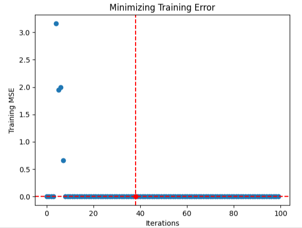
图9:可视化深度神经网络的优化
过拟合测试
过拟合是一种不希望出现的现象,即我们的模型从所给的数据中学习到了无意义的特征表示。这种情况之所以不受欢迎,是因为处于这种状态的模型预测准确性会很低。我们可以通过将模型与较弱的学习器以及类似神经网络的默认实例进行比较,来判断模型是否过拟合。如果我们的模型正在学习数据中的噪声,而未能捕捉到数据中的有效信号,那么它的表现将不如那些性能较弱的学习器。然而,即使我们的模型超越了性能较弱的学习器,但仍然有可能过拟合。
#Testing for overfitting
#Benchmark
benchmark = LinearRegression()

#Default
default_nn = MLPRegressor(max_iter=500)

#Randomized NN
random_search_nn = MLPRegressor(hidden_layer_sizes=tuner.best_params_["hidden_layer_sizes"],
                         early_stopping=tuner.best_params_["early_stopping"],
                         warm_start=tuner.best_params_["warm_start"],
                         max_iter=500,
                         activation=tuner.best_params_["activation"],
                         learning_rate=tuner.best_params_["learning_rate"],
                         solver=tuner.best_params_["solver"],
                         shuffle=tuner.best_params_["shuffle"],
                         alpha=tuner.best_params_["alpha"],
                         tol=tuner.best_params_["tol"],
                         learning_rate_init=tuner.best_params_["learning_rate_init"]
                         )

#LBFGS NN
lbfgs_nn = MLPRegressor(hidden_layer_sizes=tuner.best_params_["hidden_layer_sizes"],
                         early_stopping=tuner.best_params_["early_stopping"],
                         warm_start=tuner.best_params_["warm_start"],
                         max_iter=500,
                         activation=tuner.best_params_["activation"],
                         learning_rate=tuner.best_params_["learning_rate"],
                         solver=tuner.best_params_["solver"],
                         shuffle=tuner.best_params_["shuffle"],
                         alpha=result.x[0],
                         tol=result.x[1],
                         learning_rate_init=result.x[2]
                         )
拟合模型并评估它们的准确性。我们可以清楚地看到性能上的差异,线性回归模型的表现优于所有的深度神经网络。于是,我决定尝试拟合一个线性支持向量机(SVM)来替代。其表现比神经网络要好,但仍然未能超越线性回归模型。
#Fit the models on the training sets
benchmark = LinearRegression()
benchmark.fit(((train.loc[:,ohlc_predictors])),train.loc[:,"Price Target"])
mean_squared_error(test.loc[:,"Price Target"],benchmark.predict(((test.loc[:,ohlc_predictors]))))

#Test the default
default_nn.fit(train.loc[:,ohlc_predictors],train.loc[:,"Price Target"])
mean_squared_error(test.loc[:,"Price Target"],default_nn.predict(test.loc[:,ohlc_predictors]))

#Test the random search
random_search_nn.fit(train.loc[:,ohlc_predictors],train.loc[:,"Price Target"])
mean_squared_error(test.loc[:,"Price Target"],random_search_nn.predict(test.loc[:,ohlc_predictors]))

#Test the lbfgs nn
lbfgs_nn.fit(train.loc[:,ohlc_predictors],train.loc[:,"Price Target"])
mean_squared_error(test.loc[:,"Price Target"],lbfgs_nn.predict(test.loc[:,ohlc_predictors])
| 线性回归 | 默认NN | 随机搜索 | LBFGS NN |
|---|---|---|---|
| 2.609826e-07 | 1.996431e-05 | 0.00051 | 0.000398 |
让我们来拟合线性支持向量回归(LinearSVR)模型,它更有可能捕捉到数据中的非线性交互关系。
#From experience, I'll try LSVR
from sklearn.svm import LinearSVR
初始化模型,并使用所有数据对其进行拟合。观察发现,支持向量回归(SVR)模型的误差水平比神经网络要好,但不如线性回归模型。
#Initialize the model
lsvr = LinearSVR()

#Fit the Linear Support Vector
lsvr.fit(train.loc[:,["Open","High","Low","Close"]],train.loc[:,"Price Target"])
mean_squared_error(test.loc[:,"Price Target"],lsvr.predict(test.loc[:,["Open","High","Low","Close"]]))
导出到ONNX
开放神经网络交换格式(ONNX)使我们能够使用一种语言创建机器学习模型,然后将其共享给任何支持ONNX API的其他语言。ONNX协议正在迅速改变机器学习可利用的环境数量。ONNX使我们能够将AI无缝集成到MQL5的EA中。
#Let's export the LSVR to ONNX
import onnx
from skl2onnx import convert_sklearn
from skl2onnx.common.data_types import FloatTensorType
Create a new instance of the model.
model = LinearSVR()
基于我们现有的全部数据拟合模型。
model.fit(data.loc[:,["Open","High","Low","Close"]],data.loc[:,"Price Target"])
定义我们模型的输入形状。
#Define the input type
initial_types = [("float_input",FloatTensorType([1,4]))]
创建模型的ONNX表示形式。
#Create the ONNX representation
onnx_model = convert_sklearn(model,initial_types=initial_types,target_opset=12)
保存ONNX模型。
# Save the ONNX model
onnx.save_model(onnx_model,"EURUSD SVR M1.onnx")

图10:可视化我们的ONNX模型
在MQL5中实现
现在我们可以开始在MQL5中实现策略了。我们想要构建一个应用程序,该程序在价格高于移动平均线且AI预测价格将上涨时进行买入操作。
为了开始构建我们的应用程序,我们首先需要将刚刚创建的ONNX文件包含到EA中。
//+--------------------------------------------------------------+
//| EURUSD AI                                                    |
//+--------------------------------------------------------------+
#property copyright "Gamuchirai Ndawana"
#property link "https://metaquotes.com/en/users/gamuchiraindawa"
#property version "2.1"
#property description "Supports M1"

//+--------------------------------------------------------------+
//| Resources we need                                            |
//+--------------------------------------------------------------+
#resource "\\Files\\EURUSD SVR M1.onnx" as const uchar onnx_buffer[];
现在,我们将加载交易库。
//+--------------------------------------------------------------+
//| Libraries                                                    |
//+--------------------------------------------------------------+
#include  <Trade\Trade.mqh>
CTrade trade;
定义一些在后续保持不变的常量。
//+--------------------------------------------------------------+
//| Constants                                                    |
//+--------------------------------------------------------------+
const double  stop_percent = 1;
const int     ma_period_shift = 0;
我们将允许用户控制技术指标的参数以及程序的整体运行。
//+--------------------------------------------------------------+
//| User inputs                                                  |
//+--------------------------------------------------------------+
input group "TAs"
input double atr_multiple =2.5;             //How wide should the stop loss be?
input int    atr_period = 200;              //ATR Period
input int    ma_period = 1000;              //Moving average period

input group "Risk"
input double risk_percentage= 0.02;         //Risk percentage (0.01 - 1)
input double profit_target = 1.0;           //Profit target
现在,我们来定义全部所需的全局变量。
//+--------------------------------------------------------------+
//| Global variables                                             |
//+--------------------------------------------------------------+
double position_size = 2;
int lot_multiplier = 1;
bool  buy_break_even_setup = false;
bool  sell_break_even_setup = false;
double up_level = 0.03;
double down_level = -0.03;
double min_volume,max_volume_increase, volume_step, buy_stop_loss, sell_stop_loss,ask, bid,atr_stop,mid_point,risk_equity;
double take_profit = 0;
double close_price[3];
double moving_average_low_array[],close_average_reading[],moving_average_high_array[],atr_reading[];
long   min_distance,login;
int    ma_high,ma_low,atr,close_average;
bool   authorized = false;
double tick_value,average_market_move,margin,mid_point_height,channel_width,lot_step;
string currency,server;
bool all_closed =true;
long onnx_model;
vectorf onnx_output = vectorf::Zeros(1);
ENUM_ACCOUNT_TRADE_MODE account_type;
我们的EA将首先检查用户是否已允许其对该账户进行交易,然后会尝试加载ONNX模型,最后,如果到目前为止一切顺利,我们将加载技术指标。
//+------------------------------------------------------------------+
//| On initialization                                                |
//+------------------------------------------------------------------+
int OnInit()
  {

//--- Authorization
   if(!auth())
     {
      return(INIT_FAILED);
     }

//--- Load the ONNX model
if(!load_onnx())
   {
      return(INIT_FAILED);
   }

//--- Everything went fine
   else
     {
      load();
      return(INIT_SUCCEEDED);
     }
  }
如果EA不再使用,我们将释放分配给ONNX模型的内存。
//+------------------------------------------------------------------+
//| On deinitialization                                              |
//+------------------------------------------------------------------+
void OnDeinit(const int reason)
  {
      OnnxRelease(onnx_model);
  }
每当接收到更新的价格数据时,我们将更新全局市场变量,如果没有开仓,那么就会检查交易信号。否则,我们将更新追踪止损(trailing stop loss)。
//+------------------------------------------------------------------+
//| On every tick                                                    |
//+------------------------------------------------------------------+
void OnTick()
  {
//On Every Function Call
   update();
   static datetime time_stamp;
   datetime time = iTime(_Symbol,PERIOD_CURRENT,0);
   Comment("AI Forecast: ",onnx_output[0]);

//On Every Candle
   if(time_stamp != time)
     {

      //Mark the candle
      time_stamp = time;

      OrderCalcMargin(ORDER_TYPE_BUY,_Symbol,min_volume,ask,margin);
      calculate_lot_size();
      if(PositionsTotal() == 0)
        {
         check_signal();
        }
     }

//--- If we have positions, manage them.
   if(PositionsTotal() > 0)
     {
      check_atr_stop();
      check_profit();
     }
  }


//+------------------------------------------------------------------+
//| Check if we have any valid setups, and execute them              |
//+------------------------------------------------------------------+
void check_signal(void)
  {
  //--- Get a prediction from our model
  model_predict();
     if(onnx_output[0] > iClose(Symbol(),PERIOD_CURRENT,0))
      {
         if(above_channel())
           {
               check_buy();
           }
      }

      else
         if(below_channel())
           {
             if(onnx_output[0] < iClose(Symbol(),PERIOD_CURRENT,0))
               {
                  check_sell();
                }
           }
  }
该函数负责更新我们所有的全局市场变量。
//+------------------------------------------------------------------+
//| Update our global variables                                      |
//+------------------------------------------------------------------+
void update(void)
  {
//--- Important details that need to be updated everytick
   ask = SymbolInfoDouble(_Symbol,SYMBOL_ASK);
   bid = SymbolInfoDouble(_Symbol,SYMBOL_BID);
   buy_stop_loss = 0;
   sell_stop_loss = 0;
   check_price(3);
   CopyBuffer(ma_high,0,0,1,moving_average_high_array);
   CopyBuffer(ma_low,0,0,1,moving_average_low_array);
   CopyBuffer(atr,0,0,1,atr_reading);
   ArraySetAsSeries(moving_average_high_array,true);
   ArraySetAsSeries(moving_average_low_array,true);
   ArraySetAsSeries(atr_reading,true);
   risk_equity = AccountInfoDouble(ACCOUNT_BALANCE) * risk_percentage;
   atr_stop = (((min_distance + (atr_reading[0]* 1e5) * atr_multiple) * _Point));
   mid_point = (moving_average_high_array[0] + moving_average_low_array[0]) / 2;
   mid_point_height = close_price[0] - mid_point;
   channel_width = moving_average_high_array[0] - moving_average_low_array[0];
  }
现在,我们必须定义一个函数,该函数将确保运行应用程序。如果禁止运行应用程序,该函数将向用户提供操作说明,并返回false以终止初始化过程。
//+------------------------------------------------------------------+
//| Check if the EA is allowed to be run                             |
//+------------------------------------------------------------------+
bool auth(void)
  {
   if(!TerminalInfoInteger(TERMINAL_TRADE_ALLOWED))
     {
      Comment("Press Ctrl + E To Give The Robot Permission To Trade And Reload The Program");
      return(false);
     }

   else
      if(!MQLInfoInteger(MQL_TRADE_ALLOWED))
        {
         Comment("Reload The Program And Make Sure You Clicked Allow Algo Trading");
         return(false);
        }

   return(true);
  }
在初始化过程中,我们需要一个函数来负责加载所有的技术指标并获取重要的市场详情。这个加载函数(load function)能完成这些任务,并且由于它引用了全局变量,所以其返回类型将是void(即无返回值)。
//+---------------------------------------------------------------------+
//| Load our needed variables                                           |
//+---------------------------------------------------------------------+
void load(void)
  {
//Account Info
   currency = AccountInfoString(ACCOUNT_CURRENCY);
   server = AccountInfoString(ACCOUNT_SERVER);
   login = AccountInfoInteger(ACCOUNT_LOGIN);

//Indicators
   atr = iATR(_Symbol,PERIOD_CURRENT,atr_period);
   ma_high = iMA(_Symbol,PERIOD_CURRENT,ma_period,ma_period_shift,MODE_EMA,PRICE_HIGH);
   ma_low = iMA(_Symbol,PERIOD_CURRENT,ma_period,ma_period_shift,MODE_EMA,PRICE_LOW);

//Market Information
   min_volume = SymbolInfoDouble(_Symbol,SYMBOL_VOLUME_MIN);
   max_volume_increase = SymbolInfoDouble(_Symbol,SYMBOL_VOLUME_MAX) / SymbolInfoDouble(_Symbol,SYMBOL_VOLUME_MIN);
   min_distance = SymbolInfoInteger(_Symbol,SYMBOL_TRADE_STOPS_LEVEL);
   tick_value = SymbolInfoDouble(_Symbol,SYMBOL_TRADE_TICK_VALUE_PROFIT) * min_volume;
   lot_step = SymbolInfoDouble(_Symbol,SYMBOL_VOLUME_STEP);
   average_market_move = NormalizeDouble(10000 * tick_value,_Digits);
  }
另一方面,我们的ONNX模型将通过一个单独的函数调用来加载。该函数将从之前定义的缓冲区中创建ONNX模型,并验证输入和输出的形状。
//+------------------------------------------------------------------+
//| Load our ONNX model                                              |
//+------------------------------------------------------------------+
bool load_onnx(void)
   {
      onnx_model = OnnxCreateFromBuffer(onnx_buffer,ONNX_DEFAULT);
      ulong onnx_input [] = {1,4};
      ulong onnx_output[] = {1,1};
      if(!OnnxSetInputShape(onnx_model,0,onnx_input))
         {
            Comment("[INTERNAL ERROR] Failed to load AI modules. Relode the EA.");
            return(false);
         }

      if(!OnnxSetOutputShape(onnx_model,0,onnx_output))
         {
            Comment("[INTERNAL ERROR] Failed to load AI modules. Relode the EA.");
            return(false);
         }

     return(true);
   }
现在,让我们来定义一个将从模型中获取预测结果的函数。
//+------------------------------------------------------------------+
//| Get a prediction from our model                                  |
//+------------------------------------------------------------------+
void model_predict(void)
   {
      vectorf onnx_inputs = {iOpen(Symbol(),PERIOD_CURRENT,0),iHigh(Symbol(),PERIOD_CURRENT,0),iLow(Symbol(),PERIOD_CURRENT,0),iClose(Symbol(),PERIOD_CURRENT,0)};
      OnnxRun(onnx_model,ONNX_DEFAULT,onnx_inputs,onnx_output);
   }
我们的止损点将根据真实波幅(ATR)值进行调整。具体调整方式取决于当前交易是买入交易还是卖出交易,这是帮助我们判断应该上调止损点(通过加上当前的 ATR 值)还是下调止损点(通过减去当前的 ATR 值)的主要决定因素。此外,我们还可以使用当前ATR值的倍数,以便让用户更精细地控制其风险水平。
//+------------------------------------------------------------------+
//| Update the ATR stop loss                                         |
//+------------------------------------------------------------------+
void check_atr_stop()
  {

   for(int i = PositionsTotal() -1; i >= 0; i--)
     {

      string symbol = PositionGetSymbol(i);
      if(_Symbol == symbol)
        {

         ulong ticket = PositionGetInteger(POSITION_TICKET);
         double position_price = PositionGetDouble(POSITION_PRICE_OPEN);
         double type = PositionGetInteger(POSITION_TYPE);
         double current_stop_loss = PositionGetDouble(POSITION_SL);

         if(type == POSITION_TYPE_BUY)
           {
            double atr_stop_loss = (ask - (atr_stop));
            double atr_take_profit = (ask + (atr_stop));

            if((current_stop_loss < atr_stop_loss) || (current_stop_loss == 0))
              {
               trade.PositionModify(ticket,atr_stop_loss,atr_take_profit);
              }
           }

         else
            if(type == POSITION_TYPE_SELL)
              {
               double atr_stop_loss = (bid + (atr_stop));
               double atr_take_profit = (bid - (atr_stop));
               if((current_stop_loss > atr_stop_loss) || (current_stop_loss == 0))
                 {
                  trade.PositionModify(ticket,atr_stop_loss,atr_take_profit);
                 }
              }
        }
     }
  }
最后,我们需要定义两个函数,分别负责开设买入和卖出头寸,以及对应的用于平仓的函数。
//+------------------------------------------------------------------+
//| Open buy positions                                               |
//+------------------------------------------------------------------+
void check_buy()
  {
   if(PositionsTotal() == 0)
     {
      for(int i=0; i < position_size;i++)
        {
         trade.Buy(min_volume * lot_multiplier,_Symbol,ask,buy_stop_loss,0,"BUY");
         Print("Position: ",i," has been setup");
        }
     }
  }

//+------------------------------------------------------------------+
//| Open sell positions                                              |
//+------------------------------------------------------------------+
void check_sell()
  {
   if(PositionsTotal() == 0)
     {
      for(int i=0; i < position_size;i++)
        {
         trade.Sell(min_volume * lot_multiplier,_Symbol,bid,sell_stop_loss,0,"SELL");
         Print("Position: ",i," has been setup");
        }
     }
  }

//+------------------------------------------------------------------+
//| Close all buy positions                                          |
//+------------------------------------------------------------------+
void close_buy()
  {
   ulong ticket;
   int type;
   if(PositionsTotal() > 0)
     {
      for(int i = 0; i < PositionsTotal();i++)
        {
         if(PositionGetSymbol(i) == _Symbol)
           {
            ticket = PositionGetTicket(i);
            type = (int)PositionGetInteger(POSITION_TYPE);
            if(type == POSITION_TYPE_BUY)
              {
               trade.PositionClose(ticket);
              }
           }
        }
     }
  }

//+------------------------------------------------------------------+
//| Close all sell positions                                         |
//+------------------------------------------------------------------+
void close_sell()
  {
   ulong ticket;
   int type;
   if(PositionsTotal() > 0)
     {
      for(int i = 0; i < PositionsTotal();i++)
        {
         if(PositionGetSymbol(i) == _Symbol)
           {
            ticket = PositionGetTicket(i);
            type = (int)PositionGetInteger(POSITION_TYPE);
            if(type == POSITION_TYPE_SELL)
              {
               trade.PositionClose(ticket);
              }
           }
        }
     }
  }
让我们记录最近三个价格水平。
//+------------------------------------------------------------------+
//| Get the last 3 quotes                                            |
//+------------------------------------------------------------------+
void check_price(int candles)
  {
   for(int i = 0; i < candles;i++)
     {
      close_price[i] = iClose(_Symbol,PERIOD_CURRENT,i);
     }
  }
如果当前值高于移动平均线,其返回的布尔值为 true。
//+------------------------------------------------------------------+
//| Are we completely above the MA?                                  |
//+------------------------------------------------------------------+
bool above_channel()
  {
   return (((close_price[0] - moving_average_high_array[0] > 0)) && ((close_price[0] - moving_average_low_array[0]) > 0));
  }
检查我们是否低于移动平均线。
//+------------------------------------------------------------------+
//| Are we completely below the MA?                                  |
//+------------------------------------------------------------------+
bool below_channel()
  {
   return(((close_price[0] - moving_average_high_array[0]) < 0) && ((close_price[0] - moving_average_low_array[0]) < 0));
  }
将所有持仓平仓。
//+------------------------------------------------------------------+
//| Close all positions we have                                      |
//+------------------------------------------------------------------+
void close_all()
  {
   if(PositionsTotal() > 0)
     {
      ulong ticket;
      for(int i =0;i < PositionsTotal();i++)
        {
         ticket = PositionGetTicket(i);
         trade.PositionClose(ticket);
        }
     }
  }
计算最优手数,以便我们的保证金等于愿意承担的风险资本金额。
//+------------------------------------------------------------------+
//| Calculate the lot size to be used                                |
//+------------------------------------------------------------------+
void calculate_lot_size()
  {
//--- This is the total percentage of the account we're willing to part with for margin, or to keep a position open in other words.
   Print("Risk Equity: ",risk_equity);

//--- Now that we're ready to part with a discrete amount for margin, how many positions can we afford under the current lot size?
//--- By default we always start from minimum lot
   position_size = risk_equity / margin;

//--- We need to keep the number of positions lower than 10
   if(position_size > 10)
     {
      //--- How many times is it greater than 10?
      int estimated_lot_size = (int)  MathFloor(position_size / 10);
      position_size = risk_equity / (margin * estimated_lot_size);
      Print("Position Size After Dividing By margin at new estimated lot size: ",position_size);
      int estimated_position_size = position_size;
      //--- Can we increase the lot size this many times?
      if(estimated_lot_size < max_volume_increase)
        {
         Print("Est Lot Size: ",estimated_lot_size," Position Size: ",estimated_position_size);
         lot_multiplier = estimated_lot_size;
         position_size = estimated_position_size;
        }
     }
  }
将持仓平仓,并检查我们是否可以再次交易。
//--- This function will help us keep track of which side we need to enter the market
void close_all_and_enter()
  {

   if(PositionSelect(Symbol()))
     {
      // Determine the type of position
      check_signal();
     }
   else
     {
      Print("No open position found.");
     }
  }
如果我们达到了利润目标,将持仓平仓以实现利润,然后检查是否可以再次入场。
//+------------------------------------------------------------------+
//| Chekc if we have reached our profit target                       |
//+------------------------------------------------------------------+
void check_profit()
  {
   double current_profit = (AccountInfoDouble(ACCOUNT_EQUITY) - AccountInfoDouble(ACCOUNT_BALANCE)) / PositionsTotal();
   if(current_profit > profit_target)
     {
      close_all_and_enter();
     }

   if((current_profit * PositionsTotal()) < (risk_equity * -1))
     {
      Comment("We've breached our risk equity, consider closing all positions");
     }
  }
最后,我们需要一个函数来将所有不盈利的交易平仓。
//+------------------------------------------------------------------+
//| Close all losing trades                                          |
//+------------------------------------------------------------------+
void close_profitable_trades()
  {
   for(int i=PositionsTotal()-1; i>=0; i--)
     {
      if(PositionSelectByTicket(PositionGetTicket(i)))
        {
         if(PositionGetDouble(POSITION_PROFIT)>profit_target)
           {
            ulong ticket;
            ticket = PositionGetTicket(i);
            trade.PositionClose(ticket);
           }
        }
     }
  }
//+------------------------------------------------------------------+
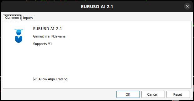
图11:我们的EA
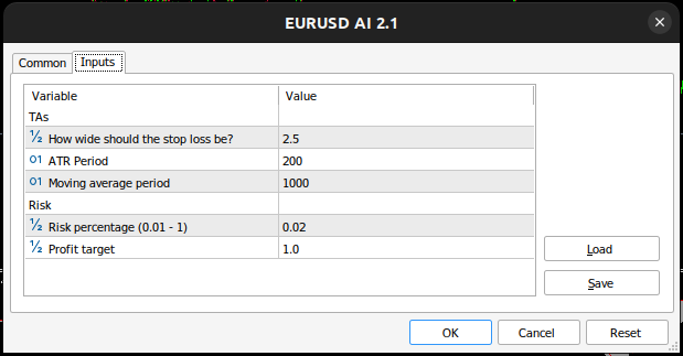
图12:我们用于测试应用程序的参数
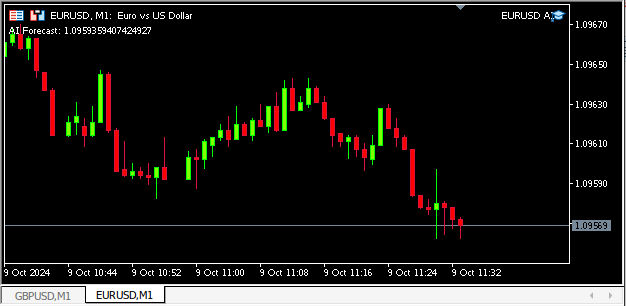
图13:我们运行中的应用
结论
尽管我们的结果并不令人满意,但并非定论。还有其他解读MACD指标的方法可能值得评估。例如,在牛市中,MACD信号线会穿过主线之上,而在熊市中,它会穿过主线之下。从这个角度看MACD指标可能会产生不同的误差指标。我们不能简单地假设所有解读MACD的方法都会产生相同的误差水平。在对MACD指标的有效性形成观点之前,我们只能合理地评估不同基于MACD的策略的有效性。
本文由MetaQuotes Ltd译自英文
原文地址: https://www.mql5.com/en/articles/16066
注意: MetaQuotes Ltd.将保留所有关于这些材料的权利。全部或部分复制或者转载这些材料将被禁止。
本文由网站的一位用户撰写,反映了他们的个人观点。MetaQuotes Ltd 不对所提供信息的准确性负责,也不对因使用所述解决方案、策略或建议而产生的任何后果负责。

 创建 MQL5-Telegram 集成 EA 交易(第 5 部分):从 Telegram 向 MQL5 发送命令并接收实时响应