Neural networks made easy (Part 21): Variational autoencoders (VAE)

Contents
- Introduction
- 1. Architecture of the variational autoencoder
- 2. Implementation
- 3. Testing
- Conclusion
- List of references
- Programs used in the article
Introduction
We continue to study unsupervised learning methods. In the last article, we got acquainted with autoencoders. The topic of autoencoders is broad and cannot fit within one article. I would like to continue this topic and introduce you to one of autoencoder modifications — variational autoencoders.
1. Architecture of the variational autoencoder
Before moving on to studying the architecture of the variational autoencoder, let's get back to the main points that we found out in the previous article.
- An autoencoder is a neural network which is trained by the backpropagation method.
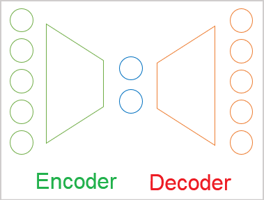
- Any autoencoder consists of Encoder and Decoder blocks.
- The encoder source data layer and the decoder result layer contain the same number of elements.
- The encoder and the decoder are joint by a "bottleneck" of the latent state which contains compressed information about the initial state.
In the process of training, we target the maximum similarity between the results of latent state decoding by the decoder and the original data. In this case, we can assert that the maximum information about the original data is encrypted in the latent state. And this data is enough to restore the original data with some probability. But the use of autoencoders is much wider than just data compression problems.
Now we will deal with the problem that was identified when using autoencoders to generate images. Let our initial data be represented by a certain cloud. During training, our model learned to perfectly restore 2 randomly selected objects A and B. Simply put, the encoder and the decoder agreed to specify 1 for the object A and 5 for the object B in the latent state. There is nothing bad in that when solving data compression problems. On the contrary, the objects are well separable, and the model can restore them.

But when the researchers tried to use autoencoders to generate images, the gap in latent state values between 2 objects proved to be a problem. Experiments showed that when the latent state values change from the object A to the object B in zones close to the objects, the decoder restored the indicated objects with some distortions. But in the middle of the interval, the decoder generated something that was not characteristic of the original data.
In other words, the latent state of autoencoders, in which the original data is encoded and compressed, can be noncontinuous or can allow some interpolation. This is the fundamental problem of autoencoders when applied to some data generation.
We are certainly not going to generate any data. But don't forget the world is constantly changing. In the process of studying the market situation, the probability of obtaining a pattern from the training set with mathematical accuracy in the future is incredibly small. However, what we want is to have the model that correctly handles the market situation and generates adequate results. Therefore, we need to find the solution of this problem for our application field, as well as for generative models.
There is no simple solution to this problem. An increase in the training sample and the use of various latent state regularization methods leads to a scaling of the problem. For example, by applying regularization, we reduce the distance between the vectors of the latent state of objects. Let's say, for our example these are the numbers 1 and 2. But there can appear an object which will be encoded as 1.5. This will confuse our decoder. Closer proximity to the overlap can make it harder to separate objects.
Increasing the training sample has a similar effect, since each state remains discrete. Furthermore, an increase in the training sample leads to an increase in the time and resources spent on training. At the same time, the autoencoder, trying to select each individual pattern of the source data, will strive to maximize the distance to the nearest neighboring state.
Unlike our model, we know that each of our discrete states is a representative of a certain class of objects. In our source data cloud, such objects are close to each other and are distributed according to a certain law of distribution. Let's add our prior knowledge to the model.

But how can we make the model return an entire range of values instead of a single value? Note that this range of values can differ in the number of discrete values and their spread. This may remind you of clustering problems. But we do not know the number of classes. This number may vary depending on the source data sample used. We need a more generic data representation model.
As already mentioned, the positioning of objects of each class in our source data cloud is subject to some distribution. Probably the most commonly used one is the normal distribution. So, let's make the assumption that each feature in the latent state at the encoder output corresponds to a normal distribution. The normal distribution is determined by two parameters: the mathematical expectation and the standard deviation. Let's ask our encoder to return not one discrete value for each feature, but two: the mathematical expectation (mean value) and the standard deviation of the distribution to which the analyzed source data pattern belongs.
But no matter how we call the values at the encoder output, for the decoder will still perceive them as numbers. Here comes the architecture of the variational autoencoder. There is no direct transmission of values between encoder and decoder in its architecture. On the contrary, we take the distribution parameters from the encoder, sample a random value from the specified distribution and input it into the decoder. Thus, as a result of processing the same source data pattern by the encoder, the decoder input may have a different vector of values, but it is always subject to the same normal distribution.
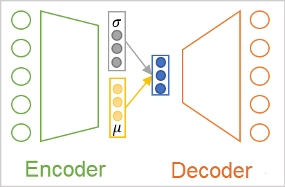
As you can see, as a result of such an operation, the decoder input will always have 2 times fewer values than the encoder output.
But here we face the problem of model training. The model is trained using the backpropagation method. One of the main requirements for this method is the differentiability of all functions along the path of the error gradient. Unfortunately, this is not true for the random number generator.
But this problem was also solved. Let's take a closer look at the properties of the normal distribution and the parameters that describe it. The normal distribution is a mathematical probability distribution centered at the point of mathematical expectation. 68% of values are at a distance of no more than the standard deviation from the center of the distribution. Therefore, a change in the mathematical expectation shifts the center of the distribution. While changing the standard deviation scales the distribution of values around the center.
Thus, to get a single value from a normal distribution with the given parameters, we can generate a value for a standard normal distribution with mathematical expectation "0" and standard deviation "1". Then the resulting value is multiplied by the given standard deviation and added to the given mathematical expectation. This approach is referred to as the reparameterization trick.
![]()
As a result, we generate a random value from the standard normal distribution in the forward pass and save it. Then we input a corrected vector with the specified parameters into the decoder. In the backpropagation pass, we easily pass the error gradient to the encoder through addition and multiplication operations, which are easily differentiated. The non-differentiable random value generator is not used in our model.
It would seem that we have put together the puzzle and bypassed all the pitfalls. But practical experiments have shown that the model does not want to play according to our new rules. Instead of learning more complex rules with new inputs, the autoencoder reduced the standard deviation features to 0 during the learning process. Multiplied by 0, our random variable has no effect, and the decoder receives a discrete value of the mathematical expectation as the input. By bringing the standard deviation features down to 0, the model nullifies all the above efforts and gets back to exchanging discrete values between the encoder and the decoder.
To make the model work according to our rules, we need to introduce additional rules and restrictions. First, we indicate to our model that the mathematical expectation and standard deviation features should correspond as much as possible to the parameters of the standard normal distribution. We can implement this by adding an additional deviation penalty. The Kullback–Leibler divergence was chosen as a measure of such a deviation. We will not dive into mathematical calculations now. So, here is the result of the error for empirical values deviating from the normal distribution parameters. We will use this function to regularize the values of the latent state. In practice, we will add its value to the latent state error.

Thus, each time penalizing the model when the feature parameters deviate from the reference (in this case, from the standard distribution), we will force the model to bring the distribution parameters of each feature closer to the parameters of the standard distribution (the mathematical expectation of 0 and the standard deviation of 1).
It must be said here that such "pulling" of features at the encoder output will go against the main problem — extracting features of individual objects. The added regularization will pull all features to the reference values with the same force. I.e., it will try to make the parameters the same. At the same time, the decoder error gradient will try to separate features of different objects as much as possible. There is clearly a conflict of interest between the 2 tasks performed. So, the model must find a balance in solving the problems. But the balance will not always meet our expectations. To control this equilibrium point, we will introduce an additional hyperparameter into the model. It will control the influence of the Kullback–Leibler divergence on the overall result.
2. Implementation
After considering the theoretical aspects of the variational autoencoder algorithm, we can move on to the practical part. To implement the encoder and decoder of the variational autoencoder, we again will use fully connected neural layers from the library created earlier. To implement a full-fledged variational autoencoder, we need a block for operating with the latent state. In this block, we will implement all the above innovations of the variational autoencoder.
To preserve the general approach to organizing neural networks in our library, we will wrap the entire latent state processing algorithm in a separate neural layer CVAE. Before proceeding with the implementation of the class, let's create kernels to implement the functionality on the OpenCL side of the device.
Let's start with the feed-forward kernel. We input into the layer parameters describing the normal distribution for the latent state features. There is one caveat. The mathematical expectation can take any value. But the standard deviation can only take non-negative values. If we used different neural layers to generate parameters, we could use different neuron activation functions. But our library architecture only allows the creation of linear models. At the same time, only one activation function can be used within one neural layer.
Again, the model does not care how the value is called. It simply executes the mathematical formulas. This is important only for us, as it allowed the correct construction of the model. Pay attention to the Kullback-Leibler divergence formula above. It uses the variance and its logarithm. The variance of a distribution is equal to the square of the standard deviation and may only be non-negative. Its logarithm can take both positive and negative values. Take a look at the graph of the natural logarithm of the squared argument: the point of intersection of the abscissa line by the function graph is exactly at 1. This value is the target for the standard deviation. Moreover, for the interval of function values from -1 to 1, the function argument takes values from 0.6 to 1.6, which satisfies our expectations for the standard deviation.

Thus, we will INSTRUCT the model encoder to output the mathematical expectation and the natural logarithm of the distribution variance. We can use the hyperbolic tangent as the activation function of the neural layer, since the range of its values satisfies our expectations for both the mathematical expectation of the distribution and the logarithm of its variance.
So, the conceptual approach is clear. Now, let us move on to programming our functions. We will start with the feed-forward kernel VAE_FeedForward. The kernel received pointers to three data buffers in parameters. Two of them contain the original data and one is the result buffer. On the OpenCL side, there is no pseudo-random number generator. Therefore, we will sample the elements of the standard distribution on the side of the main program. Then we will pass them by the "random" buffer to the feed-forward kernel.
The second source data buffer will contain the results of the encoder. As you probably already guessed, the vector of mathematical expectations and the vector of logarithms of the variance will be contained in the same buffer "inputs".
Now, we only have to implement the reparameterization trick in the kernel body. Do not forget that instead of the standard deviation, the encoder provides the logarithm of the dispersion. Therefore, before performing the trick, we need to get the standard deviation value.
The inverse of the natural logarithm is the exponential function. We can find the variance using this function. By extracting the square root of the variance, we get the standard deviation. Optionally, using the property of powers, we can simply take the exponent of half the logarithm of the variance, which will also give us the standard deviation.
![]()
In the body of the feed-forward kernel, we first determine the identifier of the current thread and the total number of running threads, which will serve as pointers in the source and result buffers to the required cells. Then perform the reparameterization trick using the standard deviation obtained from the logarithm of the variance. Write the result to the corresponding element of the result buffer and exit the kernel.
__kernel void VAE_FeedForward(__global float* inputs,
                              __global float* random,
                              __global float* outputs
                             )
  {
   uint i = (uint)get_global_id(0);
   uint total = (uint)get_global_size(0);
   outputs[i] = inputs[i] + exp(0.5f * inputs[i + total]) * random[i];
  }
So, the feed-forward kernel algorithm is quite simple. Next, we move on to organizing the backpropagation pass on the OpenCL context side. Our latent state layer of the variational autoencoder will not contain trainable parameters. Therefore, the entire backpropagation process will consist in organizing the transmission of the error gradient from the decoder to the encoder. This will be implemented in the VAE_CalcHiddenGradient kernel.
When implementing this kernel, remember that during the feed-forward pass we took two elements from the encoder result vector and after reparameterization trick passed one feature as the input into the decoder. Therefore, we must take one error gradient from the decoder and distribute it to two corresponding encoder elements.
Well, for mathematical expectation everything is simple (when adding, the error gradient is fully transferred to both terms). But for the variance logarithm, we are dealing with the derivative of a complex function.

But there is also the other side of the coin. In order to make the model work according to our rules, we introduced the Kullback-Leibler divergence. And now we will add the error gradient of the deviation of distribution parameters from the standard distribution reference values to the error gradient received from the decoder.
Let's look at the implementation of the kernel VAE_CalcHiddenGradient. The kernel receives in parameters pointers to four data buffers and one constant. Three of the received buffers carry the original information and one buffer is used for recording the results of the gradients and transferring them to the encoder level.
- inputs are the results of the encoder feed-forward. The buffer contains mathematical expectation values and logarithms of the feature variance.
- random — values of standard deviation elements used in the feed-forward pass
- gradient — error gradients received from the decoder
- inp_grad — result buffer to write error gradients passed to the encoder
- kld_mult — discrete value of the coefficient of influence of the Kullback–Leibler divergence on the total result
In the kernel body, we first determine the serial number of the current thread and the total number of running kernel threads. These values are used as pointers to the required elements of the input and result buffers.
Next, determine the value of the Kullback-Leibler divergence. Note that we strive to minimize the distance between the empirical and the reference distributions, i.e. reduce it to 0. This means that the error will be equal to the deviation value with the opposite sign. To eliminate unnecessary operations, simply remove the minus sign in front of the formula used to determine the deviation. Adjust the value by the coefficient of influence of divergence on the result.
Next, we will pass the error gradient to the encoder level. Here we will pass the sum of two gradients for each distribution parameter, according to the derivatives of the above functions.
__kernel void VAE_CalcHiddenGradient(__global float* inputs,
                                     __global float* inp_grad,
                                     __global float* random,
                                     __global float* gradient,
                                     const float kld_mult
                                    )
  {
   uint i = (uint)get_global_id(0);
   uint total = (uint)get_global_size(0);
   float kld = kld_mult * 0.5f * (inputs[i + total] - exp(inputs[i + total]) - pow(inputs[i], 2.0f) + 1);
   inp_grad[i] = gradient[i] + kld * inputs[i];
   inp_grad[i + total] = 0.5f * (gradient[i] * random[i] * exp(0.5f * inputs[i + total]) -
                                 kld * (1 - exp(inputs[i + total]))) ;
  }
We complete operations with the OpenCL program, and we move on to the implementation of the functionality on the main program side. We start by creating a new neural layer class CVAE derived from the neural layer base class CNeuronBaseOCL.
In this class, we add one variable m_fKLD_Mult to store the Kullback-Leibler coefficient of influence on the overall result and the SetKLDMult method to specify it. We also create an additional buffer m_cRandom to write random values of the standard deviation. The values will be sampled using the standard library for statistics and mathematical operations "Math\Stat\Normal.mqh".
In addition, to implement our functionality, we will override the feed-forward and backpropagation methods. Also, we will override methods for working with files.
class CVAE : public CNeuronBaseOCL
  {
protected:
   float             m_fKLD_Mult;
   CBufferDouble*    m_cRandom;

   virtual bool      feedForward(CNeuronBaseOCL *NeuronOCL);
   virtual bool      updateInputWeights(CNeuronBaseOCL *NeuronOCL) { return true; }

public:
                     CVAE();
                    ~CVAE();
   virtual bool      Init(uint numOutputs, uint myIndex, COpenCLMy *open_cl,
                          uint numNeurons, ENUM_OPTIMIZATION optimization_type, uint batch);
   //---
   virtual void      SetKLDMult(float value) { m_fKLD_Mult = value;}
   virtual bool      calcInputGradients(CNeuronBaseOCL *NeuronOCL);
   //---
   virtual bool      Save(int const file_handle);
   virtual bool      Load(int const file_handle);
   //---
   virtual int       Type(void)        const                      {  return defNeuronVAEOCL; }
  };
The constructor and destructor of a class are quite simple. In the first one, we just set the initial value of our new variable and initialize the data buffer instance to work with a sequence of random variables.
CVAE::CVAE()   : m_fKLD_Mult(0.01f)
  {
   m_cRandom = new CBufferDouble();
  }
In the class destructor, we delete the object of the buffer created in the constructor.
CVAE::~CVAE()
  {
   if(!!m_cRandom)
      delete m_cRandom;
  }
The class instance initialization method is not complicated. Actually, almost all the object initialization functionality is implemented by the method of the parent class. It implements all the necessary controls and functionality for initializing inherited objects. So, we only call the parent class method in our variational encoder class method. After its successful execution, initialize the buffer for working with a random sequence. We create for it a buffer in the OpenCL context memory.
bool CVAE::Init(uint numOutputs,

                uint myIndex,
                COpenCLMy *open_cl,

                uint numNeurons,
                ENUM_OPTIMIZATION optimization_type,

                uint batch)
  {
   if(!CNeuronBaseOCL::Init(numOutputs, myIndex, open_cl, numNeurons, optimization_type, batch))
      return false;
//---
   if(!m_cRandom)
     {
      m_cRandom = new CBufferDouble();
      if(!m_cRandom)
         return false;
     }
   if(!m_cRandom.BufferInit(numNeurons, 0.0))
      return false;
   if(!m_cRandom.BufferCreate(OpenCL))
      return false;
//---
   return true;
  }
Let's start the implementation of the main functionality of the class with the feed-forward pass CVAE::feedForward. Similar to other neural layer methods, this method received in the parameters a pointer to the object of the previous neural layer. This is followed by a control block. It primarily checks the validity of the pointers to used objects. After that, check the sizes of the received initial data. The number of elements in the previous layer result buffer must be a multiple of 2 and must be two times larger than the result buffer of the neural layer being created. Such a strict correspondence is required by the architecture of the variational autoencoder. The encoder should return two values for each feature, describing the mathematical expectation and standard deviation of the distribution of each feature.
bool CVAE::feedForward(CNeuronBaseOCL *NeuronOCL)
  {
   if(!OpenCL || !NeuronOCL || !m_cRandom)
      return false;
   if(NeuronOCL.Neurons() % 2 != 0 ||
      NeuronOCL.Neurons() / 2 != Neurons())
      return false;
After successfully checks, implement sampling of random values of the standard deviation and transfer their values to the appropriate buffer.
   double random[];
   if(!MathRandomNormal(0, 1, m_cRandom.Total(), random))
      return false;
   if(!m_cRandom.AssignArray(random))
      return false;
   if(!m_cRandom.BufferWrite())
      return false;
Pass the generated values to the OpenCL context memory for further processing.
Next, we implement the call of the corresponding kernel. First, we pass pointers to the data buffers used by the kernel. Note that we only passed the generated case buffer to the context memory. We expect that all other used data buffers are already in the context memory. If you have not previously created buffers in the context memory or have made any changes to the buffer data on the main program side, then before passing the buffer pointers to the kernel parameters, you must pass the data to the OpenCL context memory. You should always remember that an OpenCL program operates only on its context memory, without accessing the computer's global memory. Even if you are using an integrated graphics card or the OpenCL library on the processor.
   if(!OpenCL.SetArgumentBuffer(def_k_VAEFeedForward, def_k_vaeff_inputs, NeuronOCL.getOutput().GetIndex()))
      return false;
   if(!OpenCL.SetArgumentBuffer(def_k_VAEFeedForward, def_k_vaeff_random, m_cRandom.GetIndex()))
      return false;
   if(!OpenCL.SetArgumentBuffer(def_k_VAEFeedForward, def_k_vaeff_outputd, Output.GetIndex()))
      return false;
At the end of the method, specify the dimension of tasks, the offset for each dimension, and call the method to enqueue the kernel for execution.
   uint off_set[] = {0};
   uint NDrange[] = {Neurons()};
   if(!OpenCL.Execute(def_k_VAEFeedForward, 1, off_set, NDrange))
      return false;
//---
   return true;
  }
Do not forget to check the result at each step.
After successful completion of the operations, exit the method with true.
The feed forward passage is followed by the backpropagation. Previously, we implemented the backward pass using several methods. First, we used calcOutputGradients, calcHiddenGradients and calcInputGradients to implement the calculation and passing of the error gradient sequentially through our entire model from the neural output layer to the input data layer. Then, we use updateInputWeights to change the trained parameters towards the anti-gradient.
Our neural layer for working with the latent layer of the variational autoencoder does not contain trainable parameters. Therefore, we will override the last method of parameter optimization with a stub that will always return true every time the method is called.
In fact, for the normal implementation of the back pass process in the class, we should only redefine the calcInputGradients method. Although functionally the forward and backward pass methods have a reverse data flow direction, the content of the methods is quite similar. This is because the functionality of the algorithms is implemented on the OpenCL context site. On the side of the main program, we are only doing preparatory work to call the kernels. They will be called according to a single template.
As in the feed forward method, we first check the validity of the pointers to the objects being used. We do not re-pass data to the OpenCL context. But if you are not sure that all the necessary information is in the context memory, it is better to pass it again to the OpenCL context memory now. After that we can pass parameters to the kernel.
After the successful transfer of parameters, there is a block of operations to start kernel execution. First, set the size of the problems and the offset along each dimension. Then call the method which will put the kernel to the execution queue.
bool CVAE::calcInputGradients(CNeuronBaseOCL *NeuronOCL)
  {
   if(!OpenCL || !NeuronOCL)
      return false;
//---
   if(!OpenCL.SetArgumentBuffer(def_k_VAECalcHiddenGradient, def_k_vaehg_input,
                                                        NeuronOCL.getOutput().GetIndex()))
      return false;
   if(!OpenCL.SetArgumentBuffer(def_k_VAECalcHiddenGradient, def_k_vaehg_inp_grad,
                                                        NeuronOCL.getGradient().GetIndex()))
      return false;
   if(!OpenCL.SetArgumentBuffer(def_k_VAECalcHiddenGradient, def_k_vaehg_random, Weights.GetIndex()))
      return false;
   if(!OpenCL.SetArgumentBuffer(def_k_VAECalcHiddenGradient, def_k_vaehg_gradient, Gradient.GetIndex()))
      return false;
   if(!OpenCL.SetArgument(def_k_VAECalcHiddenGradient, def_k_vaehg_kld_mult, m_fKLD_Mult))
      return false;
   int off_set[] = {0};
   int NDrange[] = {Neurons()};
   if(!OpenCL.Execute(def_k_VAECalcHiddenGradient, 1, off_set, NDrange))
      return false;
//---
   return true;
  }
We check the results of all operations and exit the method.
This concludes the implementation of the main functionality of the class. But there is another important functionality — operations with files. Therefore, we will supplement the functionality of the class with these methods. Before proceeding to writing class methods, let's think about which information we need to save in order to successfully restore the model performance. In this class, we have created only one variable and one data buffer. The buffer contents are filled with random values on each forward pass. Therefore, there is no need for us to save this data. The value of the variable is a hyperparameter and we need to save it.
Thus, our object save method will contain only 2 operations:
- call a similar parent class method, which performs all the necessary controls and saves inherited objects
- save the hyperparameter of the Kullback–Leibler divergence influence on the overall result.
bool CVAE::Save(const int file_handle)
  {
//---
   if(!CNeuronBaseOCL::Save(file_handle))
      return false;
   if(FileWriteFloat(file_handle, m_fKLD_Mult) < sizeof(m_fKLD_Mult))
      return false;
//---
   return true;
  }
Do not forget to check the operation result. After successful completion of all operations, exit the method with the true result.
To restore the model performance, the saved data from the file is read in strict accordance with the data writing order. We first call a similar parent class method. It contains all the necessary controls and loads inherited objects.
bool CVAE::Load(const int file_handle)
  {
   if(!CNeuronBaseOCL::Load(file_handle))
      return false;
   m_fKLD_Mult=FileReadFloat(file_handle);
After the successful execution of the parent class method, read the hyperparameter values from the file and write it to the corresponding variable. But unlike the data saving method, the data loading method does not end here. True, there is no more information in the file to load into this class. But to organize its correct operation, we need to initialize the buffer to work with random variables of the correct size. Create a buffer with a size equal to the loaded buffer of the current neural layer results (it was loaded by the parent class method). Also create the relevant buffer in the OpenCL context memory.
   if(!m_cRandom)
     {
      m_cRandom = new CBufferDouble();
      if(!m_cRandom)
         return false;
     }
   if(!m_cRandom.BufferInit(Neurons(), 0.0))
      return false;
   if(!m_cRandom.BufferCreate(OpenCL))
      return false;
//---
   return true;
  }
After successful completion of all operations, exit the method with the true result.
This concludes the variational autoencoder latent state processing class. The complete code of all methods and classes is available in the attachment below.
Our new class is ready. But our dispatching class that organizes the operation of the neural network still does not know anything about it. So, go to NeuroNet.mqh and find the CNet class.
First, go to the class constructor and describe the procedure for creating a new neural layer. Also, increase the number of used OpenCL kernels and declare two new kernels.
CNet::CNet(CArrayObj *Description)  :  recentAverageError(0),
                                       backPropCount(0)
  {
  .................
  .................
//---
   for(int i = 0; i < total; i++)
     {
  .................
  .................
      if(CheckPointer(opencl) != POINTER_INVALID)
        {
         CNeuronBaseOCL *neuron_ocl = NULL;
         CNeuronConvOCL *neuron_conv_ocl = NULL;
         CNeuronProofOCL *neuron_proof_ocl = NULL;
         CNeuronAttentionOCL *neuron_attention_ocl = NULL;
         CNeuronMLMHAttentionOCL *neuron_mlattention_ocl = NULL;
         CNeuronDropoutOCL *dropout = NULL;
         CNeuronBatchNormOCL *batch = NULL;
         CVAE *vae = NULL;
         switch(desc.type)
           {
  .................
  .................
            //---
            case defNeuronVAEOCL:
               vae = new CVAE();
               if(!vae)
                 {
                  delete temp;
                  return;
                 }
               if(!vae.Init(outputs, 0, opencl, desc.count, desc.optimization, desc.batch))
                 {
                  delete vae;
                  delete temp;
                  return;
                 }
               if(!temp.Add(vae))
                 {
                  delete vae;
                  delete temp;
                  return;
                 }
               vae = NULL;
               break;
            default:
               return;
               break;
           }
        }
      else
         for(int n = 0; n < neurons; n++)
           {
  .................
  .................
           }
      if(!layers.Add(temp))
        {
         delete temp;
         delete layers;
         return;
        }
     }
//---
   if(CheckPointer(opencl) == POINTER_INVALID)
      return;
//--- create kernels
   opencl.SetKernelsCount(32);
  .................
  .................
   opencl.KernelCreate(def_k_VAEFeedForward, "VAE_FeedForward");
   opencl.KernelCreate(def_k_VAECalcHiddenGradient, "VAE_CalcHiddenGradient");
//---
   return;
  }
Implement similar changes to the model loading method CNet::Load. I will not repeat the code in this article. The entire code is provided in the attachment.
Next, add pointers to the new class in the CLayer::CreateElement and CLayer::Load methods.
Finally, add new class pointers to the dispatcher methods of the base neural layer CNeuronBaseOCL FeedForward, calcHiddenGradients and UpdateInputWeights.
After making all the necessary additions, we can start implementing and testing the model. The full code of all classes and their methods is available in the attachment.
3. Testing
To test the operation of the variational autoencoder, we will use the model from the previous articles. Saved it in a new file "vae.mq5". In that model, the encoder returned 2 values on the 5th neural layer. To properly organize the operation of the variational autoencoder, I increased the layer size at the encoder output to 4 neurons. I also inserted our new neural layer working with the latent state of the variational autoencoder as the 6th neuron. The model was trained on EURUSD data and the H1 timeframe without changing the parameters. The last 15 years were used as the time period for model training. A comparative graph of the learning dynamics of multilayer and variational autoencoders is shown in the figure below.

As you can see, according to the results of model training, the variational autoencoder showed a significantly lower data recovery error throughout the entire training period. In addition, the variational autoencoder showed a higher error reduction dynamics.
Based on the test results, we can conclude that for solving the problems of extracting time series features using the example of EURUSD price dynamics, variational autoencoders have great potential in extracting individual pattern description features.
Conclusion
In this article, we got acquainted with the variational autoencoder algorithm . We built a class to implement the variational autoencoder algorithm. We also conducted test training of the variational autoencoder model on real historical data. The test results demonstrate the consistency of the variational autoencoder model when used as a preliminary training for models intended at extracting individual features of describing the market situation. The results of such training can be used to create trading patterns which can further be trained using supervised learning methods.
List of references
- Neural networks made easy (Part 14): Data clustering
- Neural networks made easy (Part 15): Data clustering using MQL5
- Neural networks made easy (Part 16): Practical use of clustering
- Neural networks made easy (Part 17): Dimensionality reduction
- Neural networks made easy (Part 18): Association rules
- Neural networks made easy (Part 19): Association rules using MQL5
- Neural networks made easy (Part 20): Autoencoders
- Tutorial on Variational Autoencoders
- Intuitively Understanding Variational Autoencoders
- Tutorial - What is a variational autoencoder?
Programs used in the article
| # | Name | Type | Description |
|---|---|---|---|
| 1 | vae.mq5 | EA | Variational autoencoder learning Expert Advisor |
| 2 | vae2.mq5 | EA | EA for preparing data for visualization |
| 3 | VAE.mqh | Class library | Variational autoencoder latent layer class library |
| 4 | NeuroNet.mqh | Class library | A library of classes for creating a neural network |
| 5 | NeuroNet.cl | Code Base | OpenCL program code library |
Translated from Russian by MetaQuotes Ltd.
Original article: https://www.mql5.com/ru/articles/11206
Warning: All rights to these materials are reserved by MetaQuotes Ltd. Copying or reprinting of these materials in whole or in part is prohibited.
This article was written by a user of the site and reflects their personal views. MetaQuotes Ltd is not responsible for the accuracy of the information presented, nor for any consequences resulting from the use of the solutions, strategies or recommendations described.

 CCI indicator. Three transformation steps
 Neural networks made easy (Part 22): Unsupervised learning of recurrent models
 Data Science and Machine Learning (Part 07): Polynomial Regression
- Free trading apps
- Over 8,000 signals for copying
- Economic news for exploring financial markets
You agree to website policy and terms of use
Hello,
when I compile the NeuroNet.mqh file attached at the end of this article, I get 6 errors, all of them reporting: 'pow' - ambiguous call to overloaded function. Particular lines are 3848, 4468, 6868. Can somebody help me with that please?
Thank you very much
Hello,
when I compile the NeuroNet.mqh file attached at the end of this article, I get 6 errors, all of them reporting: 'pow' - ambiguous call to overloaded function. Particular lines are 3848, 4468, 6868. Can somebody help me with that please?
Thank you very much