MQL5 のIterated Function Systems (IFS) でフラクタルを生成 - MetaTrader 5のためのエキスパート

イントロダクション

Iterated Function System (IFS)では、自己相似の生成ができるプログラムがあります。例として、 Fractint、 Fractal Designer 、 IFS Matlab Generatorを見てみましょう。 MQL5言語とグラフィックオブジェクトの機能によって、 MetaTrader 5でこれらの機能を使うことができます。

Dmitry (Integer)で開発されたcIntBMPライブラリ で、これまでにないグラフィックの機能とシンプルな画像の生成が可能です。このライブラリは MetaQuotes Software Corpで特別な賞をとっています。

今回は、 cIntBMP ライブラリの機能を使います。さらに、Iterated Function Systemsを使って、フラクタルの生成アルゴリズムを考察します。

1. 平面のアフィン変換

２次元のアフィン変換とは写像 の一つである。一般的に、２次元のアフィン変換は行列と  ベクトルで決定されます。アフィン変換によって移された点 は (x,y) を行列で線形変換したのちにベクトルで平行移動した点として定義されます:

アフィン変換で使われる行列は正則でなければなりません。。  アフィン変換は一般の行列変換と同様にベクトルのサイズを倍します。

アフィン変換は幾何的構造を変えません。(線は線に変換されます。)　ATは オブジェクトをシンプルに"変形"（回転、拡大縮小、並進など）します。

アフィン平面変換の例:

1) 平面の回転 の アングル:

2) "平面のスケーリング" と 係数 (X と Y axes):

3) ベクトルによる平面の変換 :

縮小写像が鍵です。 (Hutchinson の結果参照)。

と が と にします。 は距離です。 (例 ユークリッド距離: )。 アフィン変換は下記の条件時 縮小写像と呼ばれます。 。

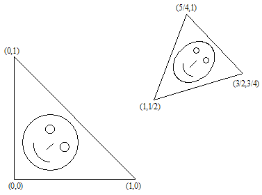
アフィン変換の例です:

結果:

2. 単純変形

フラクタルは下記の方法で構築します: ある単純な幾何的なオブジェクト (セクション、三角、四角)をN個に分割し、そのうちのM個を縮小写像"に使います。 ( N=Mの場合、整数次元になります。) この作業をそれぞれのピースで何度も繰り返します。

古典的フラクタル:

セクション:

• Triadic Koch Curve, N=3, M=4;
• Cantor Dust, N=3, M=2;

三角形:

• Sierpinski Gasket, N=4, M=3;

四角形:

• Sierpinski Carpet, N=9, M=8;
• Vichek fractal, N=9, M=5。

など。

フラクタルには自己相似構造の性質があります。いくつの構造は同じような変換で定義されます。アフィン変換の構造は、フラクタル構造の方式に依存しています。

後述を見れば明らかですが、唯一の問題は最初のフラクタル構造の反復を記述し、アフィン変換の集合を見つけなければならないことです。

ここに、ある集合があるとします。フラクタルの生成アルゴリズムによれば、変形し、回転させ、"特定の場所"に飛ばす必要があります。問題はアフィン転換を使ってプロセスを記述することです。つまり、行列とベクトルを見つける必要があります。

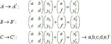
初めの集合の３点で十分であると証明すること、それらを３つのそれぞれの点に変換することは簡単です。この変換は６つの線形方程式を導き、a,b,c,d,e,f の解を求めることができます。

例 三角から変換された 三角を考えます。

線形方程式を解くことによって、 a,b,c,d,e, f の係数を求めることができます。

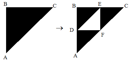
例:シェルピンスキーのギャスケット:

それぞの点の座標:

• A (0,0)
• B (0,1)
• C (1,1)
• D(0,1/2)
• E (1/2,1)
• F(1/2,1/2)
  

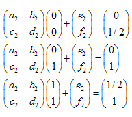
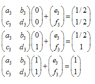
３つの変換:

1. ABC -> ADF
2. ABC -> DBE
3. ABC -> FEC
   

線形方程式は下記のようになります:

1. 
   
2. 
   
3. 
   

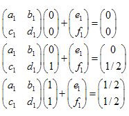
解は: , ,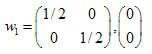

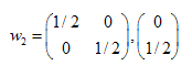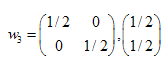
アフィン変換の係数を求められました。これにより自己相似集合を生成することができます。

3. 反復関数系を使ったフラクタルの生成

反復関数系 (IFS)は - "重み付けされた"アフィン収縮の集合です。  それぞれのIFS関数は7つの数によって定義されます: , ただし重みづけは反復プロセスがn回変換する可能性があるとき使われます。収縮の際は比例の関係にある値を定義すべきです: 。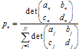

反復関係系を使ったフラクタル収縮のアルゴリズムについて考察してみましょう。 ( カオスゲーム参照)。

初めにすることは初期位置の座標を設定します。。 次に、無作為に座標を選択し、プロットします。。 そして再び、無作為に座標を選び、 プロット します。そうすると、 点の座標が得られます。

収縮の選択は"可能性"に依存しています。このプロセスを繰り返し、(例えば、~30000 ほど)　その結果を座標にプロットすると、ランダムにも関わらず構造が現れます。

これがシェルピンスキーのギャスケットの一例です:

図1. IFSで生成したシェルピンスキーのギャスケット(チャプター２)

コード:

//+------------------------------------------------------------------+
//|                                        IFS_Sierpinski_Gasket.mq5 |
//|                        Copyright 2011, MetaQuotes Software Corp. |
//|                                              https://www.mql5.com |
//+------------------------------------------------------------------+
#property copyright "Copyright 2011, MetaQuotes Software Corp."
#property link      "https://www.mql5.com"
#property version   "1.00"

//-- include file with cIntBMP class
#include <cIntBMP.mqh>

//-- Sierpinski Gasket IFS coefficients
//-- (a,b,c,d) matricies
double IFS_a[3] = {0.50,  0.50,  0.50};
double IFS_b[3] = {0.00,  0.00,  0.00};
double IFS_c[3] = {0.00,  0.00,  0.00};
double IFS_d[3] = {0.50,  0.50,  0.50};
//-- (e,f) vectors
double IFS_e[3] = {0.00,  0.00,  0.50};
double IFS_f[3] = {0.00,  0.50,  0.50};
//-- "probabilities" of transforms, multiplied by 1000
double IFS_p[3]={333,333,333};

double Probs[3]; // Probs array - used to choose IFS transforms
cIntBMP bmp;     // cIntBMP class instance
int scale=350;  // scale coefficient
//+------------------------------------------------------------------+
//| Expert initialization function                                   |
//+------------------------------------------------------------------+
int OnInit()
  {
//-- Prepare Probs array
   double m=0;
   for(int i=0; i<ArraySize(IFS_p); i++)
     {
      Probs[i]=IFS_p[i]+m;
      m=m+IFS_p[i];
     }
//-- size of BMP image
   int XSize=500;
   int YSize=400;
//-- create bmp image XSizexYSize with clrSeashell background color
   bmp.Create(XSize,YSize,clrSeashell);
//-- image rectangle
   bmp.DrawRectangle(0,0,XSize-1,YSize-1,clrBlack);

//-- point coordinates (will be used in construction of set)
   double x0=0;
   double y0=0;
   double x,y;
//-- number of points to calculate (more points - detailed image)
   int points=1500000;
//-- calculate set
   for(int i=0; i<points; i++)
     {
      // choose IFS tranform with probabilities, proportional to defined
      double prb=1000*(rand()/32767.0);
      for(int k=0; k<ArraySize(IFS_p); k++)
        {
         if(prb<=Probs[k])
           {
            // affine transformation
            x = IFS_a[k] * x0 + IFS_b[k] * y0 + IFS_e[k];
            y = IFS_c[k] * x0 + IFS_d[k] * y0 + IFS_f[k];
            // update previous coordinates
            x0 = x;
            y0 = y;
            // convert to BMP image coordinates
            // (note the Y axis in cIntBMP)
            int scX = int (MathRound(XSize/2 + (x-0.5)*scale));
            int scY = int (MathRound(YSize/2 + (y-0.5)*scale));
            // if the point coordinates inside the image, draw the dot
            if(scX>=0 && scX<XSize && scY>=0 && scY<YSize) { bmp.DrawDot(scX,scY,clrDarkBlue); }
            break;
           }
        }
     }
//-- save image to file
   bmp.Save("bmpimg",true);
//-- plot image on the chart
   bmp.Show(0,0,"bmpimg","IFS");
//---
   return(0);
  }
//+------------------------------------------------------------------+
//| Expert deinitialization function                                 |
//+------------------------------------------------------------------+
void OnDeinit(const int reason)
  {
//--- delete image from the chart
   ObjectDelete(0,"IFS");
//--- delete file
   bmp.Delete("bmpimg",true);
  }
//+------------------------------------------------------------------+

1350をスケールに設定した場合、反復の数は15000000まで増加し、初期座標をずらします:

int scX = MathRound(XSize/2 + (x-0.75)*scale);
int scY = MathRound(YSize/2 + (y-0.75)*scale);

拡大した領域を見ることが可能です。図2では自己相似構造を確認できます:

図2. シェルピンスキーのギャスケットの拡大領域

Michael Barnsleyによる、有名なバーンズリーのシダの葉を考察しましょうこちらはより複雑です。

図3. バーンズリーのシダの葉

コードは似ていますが、この場合４つのIFS 収縮を異なる重み付けで使います。

//+------------------------------------------------------------------+
//|                                                     IFS_fern.mq5 |
//|                        Copyright 2011, MetaQuotes Software Corp. |
//|                                              https://www.mql5.com |
//+------------------------------------------------------------------+
#property copyright "Copyright 2011, MetaQuotes Software Corp."
#property link      "https://www.mql5.com"
#property version   "1.00"
#include <cIntBMP.mqh>
//-- Barnsley Fern IFS coefficients
//-- (a,b,c,d) matricies
double IFS_a[4] = {0.00,  0.85,  0.20,  -0.15};
double IFS_b[4] = {0.00,  0.04, -0.26,   0.28};
double IFS_c[4] = {0.00, -0.04,  0.23,   0.26};
double IFS_d[4] = {0.16,  0.85,  0.22,   0.24};
//-- (e,f) vectors
double IFS_e[4] = {0.00,  0.00,  0.00,   0.00};
double IFS_f[4] = {0.00,  1.60,  1.60,   0.00};
//-- "probabilities" of transforms, multiplied by 1000
double IFS_p[4] = {10,     850,    70,     70};

double Probs[4];
cIntBMP bmp;
int scale=50;
//+------------------------------------------------------------------+
//| Expert initialization function                                   |
//+------------------------------------------------------------------+
int OnInit()
  {
   double m=0;
   for(int i=0; i<ArraySize(IFS_p); i++)
     {
      Probs[i]=IFS_p[i]+m;
      m=m+IFS_p[i];
     }

   int XSize=600;
   int YSize=600;

   bmp.Create(XSize,YSize,clrSeashell);

   bmp.DrawRectangle(0,0,XSize-1,YSize-1,clrBlack);

   double x0=0;
   double y0=0;
   double x,y;

   int points=250000;

   for(int i=0; i<points; i++)
     {
      double prb=1000*(rand()/32767.0);
      for(int k=0; k<ArraySize(IFS_p); k++)
        {
         if(prb<=Probs[k])
           {
            x = IFS_a[k] * x0 + IFS_b[k] * y0 + IFS_e[k];
            y = IFS_c[k] * x0 + IFS_d[k] * y0 + IFS_f[k];
            x0 = x;
            y0 = y;
            int scX = int (MathRound(XSize/2 + (x)*scale));
            int scY = int (MathRound(YSize/2 + (y-5)*scale));
            if(scX>=0 && scX<XSize && scY>=0 && scY<YSize) { bmp.DrawDot(scX,scY,clrForestGreen); }
            break;
           }
        }
     }
   bmp.Save("bmpimg",true);
   bmp.Show(0,0,"bmpimg","IFS");
//---
   return(0);
  }
//+------------------------------------------------------------------+
//| Expert deinitialization function                                 |
//+------------------------------------------------------------------+
void OnDeinit(const int reason)
  {
   ObjectDelete(0,"IFS");
   bmp.Delete("bmpimg",true);
  }
//+------------------------------------------------------------------+ 

このような複雑な構造体をたった２８個の数で定義できることは驚愕です。

スケールを150にした場合、反復の数は1250000になり、拡大した断片をみることができます。

図4. バーンズリーのシダの葉の断片

この通り、このアルゴリズムは広くあてはめることができ、異なるフラクタルを生成することも可能です。

次の例は、IFSによるシェルピンスキーのカーペットです:

//-- Sierpinski Gasket IFS coefficients
double IFS_a[8] = {0.333, 0.333, 0.333, 0.333, 0.333, 0.333, 0.333, 0.333};
double IFS_b[8] = {0.00,  0.00,  0.00,   0.00, 0.00,  0.00,  0.00,   0.00};
double IFS_c[8] = {0.00,  0.00,  0.00,   0.00, 0.00,  0.00,  0.00,   0.00};
double IFS_d[8] = {0.333, 0.333,  0.333,  0.333, 0.333,  0.333,  0.333, 0.333};
double IFS_e[8] = {-0.125, -3.375, -3.375,  3.125, 3.125, -3.375, -0.125, 3.125};
double IFS_f[8] = {6.75, 0.25, 6.75,  0.25, 6.75, 3.5, 0.25, 3.50};
//-- "probabilities", multiplied by 1000
double IFS_p[8]={125,125,125,125,125,125,125,125};

Figure 5. シェルピンスキーのカーペット

チャプター２ではIFSの係数の計算アルゴリズムを考察しました。

"フラクタルワード"を生成する方法について考察してみましょう。ロシア語では、"フラクタル"はこのようになります:

図6. ロシア語で"フラクタル"

IFS係数を見つけるには、対応する線形系を解く必要があります。解:

//-- IFS coefficients of the "Fractals" word in Russian
double IFS_a[28]=
  {
   0.00, 0.03,  0.00, 0.09, 0.00, 0.03, -0.00, 0.07, 0.00, 0.07, 0.03,  0.03,  0.03,  0.00,
   0.04, 0.04, -0.00, 0.09, 0.03, 0.03,  0.03, 0.03, 0.03, 0.00, 0.05, -0.00,  0.05,  0.00
  };

double IFS_b[28]=
  {
   -0.11, 0.00, 0.07, 0.00, -0.07, 0.00, -0.11,  0.00, -0.07,  0.00, -0.11,  0.11, 0.00, -0.14,
   -0.12, 0.12,-0.11, 0.00, -0.11, 0.11,  0.00, -0.11,  0.11, -0.11,  0.00, -0.07, 0.00, -0.07
  };

double IFS_c[28]=
  {
   0.12,  0.00,  0.08,  -0.00,  0.08,  0.00,  0.12,  0.00,  0.04,  0.00,  0.12,  -0.12, 0.00,  0.12,
   0.06,  -0.06,  0.10,  0.00,  0.12,  -0.12,  0.00,  0.12,  -0.12,  0.12, 0.00,  0.04,  0.00,  0.12
  };

double IFS_d[28]=
  {
   0.00,  0.05,  0.00,  0.07,  0.00,  0.05,  0.00,  0.07,  0.00,  0.07,  0.00,  0.00,  0.07,  0.00,
   0.00,  0.00,  0.00,  0.07,  0.00,  0.00,  0.07,  0.00,  0.00,  0.00,  0.07,  0.00,  0.07,  0.00
  };

double IFS_e[28]=
  {
   -4.58,  -5.06, -5.16, -4.70, -4.09, -4.35, -3.73, -3.26, -2.76,  -3.26, -2.22, -1.86, -2.04, -0.98,
   -0.46,  -0.76,  0.76,  0.63,  1.78,  2.14,  1.96,  3.11,  3.47,  4.27,  4.60,  4.98,   4.60, 5.24
  };

double IFS_f[28]=
  {
   1.26,  0.89,  1.52,  2.00,  1.52,  0.89,  1.43,  1.96,  1.69,  1.24,  1.43,  1.41,  1.11,  1.43,
   1.79,  1.05,  1.32,  1.96,  1.43,  1.41,  1.11,  1.43,  1.41,  1.43,  1.42,  1.16,  0.71,  1.43
  };

//-- "probabilities", multiplied by 1000
double IFS_p[28]=
  {
   35,  35,  35,  35,  35,  35,  35,  35,  35,  35,  35,  35,  35,  35,  
   35,  35,  35,  35,  35,  35,  35,  35,  35,  35,  35,  35,  35,  35
  };

結果は下記の画像になります:

図7. 自己相似文字

全ソースコードはifs_fractals.mq5にあります。

拡大すると、自己相似構造を確認できます:

図8. 拡大した図

IFSによる自己相似集合は Fractal Designerを使って構築できます。

IFSを使って、フラクタルを構築する方法を収録しました。cIntBMPライブライリによって、このプロセスは非常に簡単になっています。では、クラスを生成し、画像を良くするためにいくつか特徴を追加しましょう。

4. IFSの構造のクラス

偶然による集合の構築について疑問に思うかもしれません。偶然性の違いは、集合が不規則な構造を持っているということになります。(IFSのシダの葉の重み付け参照。) このことは綺麗な画像の生成に使われています。隣り合う色が均等に区別できるように色を設定する必要があります。

ピクセルカラーが前の値に依存している場合、ビジュアルスクリーン(配列)を使ってできます。最後に、ビジュアルスクリーンをパレットを使ってbmpにします。bmp画像自体はチャートの背景画像として描写されます。

CIFS によるEAのコードです:

//+------------------------------------------------------------------+
//|                                               IFS_Fern_color.mq5 |
//|                        Copyright 2011, MetaQuotes Software Corp. |
//|                                              https://www.mql5.com |
//+------------------------------------------------------------------+
#include <cIntBMP.mqh>
//-- Barnsley Fern IFS coefficients
double IFS_a[4] = {0.00,  0.85,  0.20,  -0.15};
double IFS_b[4] = {0.00,  0.04, -0.26,   0.28};
double IFS_c[4] = {0.00, -0.04,  0.23,   0.26};
double IFS_d[4] = {0.16,  0.85,  0.22,   0.24};
double IFS_e[4] = {0.00,  0.00,  0.00,   0.00};
double IFS_f[4] = {0.00,  1.60,  1.60,   0.00};
double IFS_p[4] = {10,     850,    70,     70};
//-- Palette
uchar Palette[23*3]=
  {
   0x00,0x00,0x00,0x02,0x0A,0x06,0x03,0x11,0x0A,0x0B,0x1E,0x0F,0x0C,0x4C,0x2C,0x1C,0x50,0x28,
   0x2C,0x54,0x24,0x3C,0x58,0x20,0x4C,0x5C,0x1C,0x70,0x98,0x6C,0x38,0xBC,0xB0,0x28,0xCC,0xC8,
   0x4C,0xB0,0x98,0x5C,0xA4,0x84,0xBC,0x68,0x14,0xA8,0x74,0x28,0x84,0x8C,0x54,0x94,0x80,0x40,
   0x87,0x87,0x87,0x9F,0x9F,0x9F,0xC7,0xC7,0xC7,0xDF,0xDF,0xDF,0xFC,0xFC,0xFC
  };
//+------------------------------------------------------------------+
//| CIFS class                                                       |
//+------------------------------------------------------------------+
class CIFS
  {
protected:
   cIntBMP           m_bmp;
   int               m_xsize;
   int               m_ysize;
   uchar             m_virtual_screen[];
   double            m_scale;
   double            m_probs[8];

public:
                    ~CIFS()                          { m_bmp.Delete("bmpimg",true); };
   void              Create(int x_size,int y_size,uchar col);
   void              Render(double scale,bool back);
   void              ShowBMP(bool back);
protected:
   void              VS_Prepare(int x_size,int y_size,uchar col);
   void              VS_Fill(uchar col);
   void              VS_PutPixel(int px,int py,uchar col);
   uchar             VS_GetPixel(int px,int py);
   int               GetPalColor(uchar index);
   int               RGB256(int r,int g,int b) const {return(r+256*g+65536*b);      }
   void              PrepareProbabilities();
   void              RenderIFSToVirtualScreen();
   void              VirtualScreenToBMP();
  };
//+------------------------------------------------------------------+
//| Create method                                                    |
//+------------------------------------------------------------------+
void CIFS::Create(int x_size,int y_size,uchar col)
  {
   m_bmp.Create(x_size,y_size,col);
   VS_Prepare(x_size,y_size,col);
   PrepareProbabilities();
  }
//+------------------------------------------------------------------+
//| Prepares virtual screen                                          |
//+------------------------------------------------------------------+
void CIFS::VS_Prepare(int x_size,int y_size,uchar col)
  {
   m_xsize=x_size;
   m_ysize=y_size;
   ArrayResize(m_virtual_screen,m_xsize*m_ysize);
   VS_Fill(col);
  }
//+------------------------------------------------------------------+
//| Fills the virtual screen with specified color                    |
//+------------------------------------------------------------------+
void CIFS::VS_Fill(uchar col)
  {
   for(int i=0; i<m_xsize*m_ysize; i++) {m_virtual_screen[i]=col;}
  }
//+------------------------------------------------------------------+
//| Returns the color from palette                                   |
//+------------------------------------------------------------------+
int CIFS::GetPalColor(uchar index)
  {
   int ind=index;
   if(ind<=0) {ind=0;}
   if(ind>22) {ind=22;}
   uchar r=Palette[3*(ind)];
   uchar g=Palette[3*(ind)+1];
   uchar b=Palette[3*(ind)+2];
   return(RGB256(r,g,b));
  }
//+------------------------------------------------------------------+
//| Draws a pixel on the virtual screen                              |
//+------------------------------------------------------------------+
void CIFS::VS_PutPixel(int px,int py,uchar col)
  {
   if (px<0) return;
   if (py<0) return;
   if (px>m_xsize) return;
   if (py>m_ysize) return;
    int pos=m_xsize*py+px;
   if(pos>=ArraySize(m_virtual_screen)) return;
   m_virtual_screen[pos]=col;
  }
//+------------------------------------------------------------------+
//| Gets the pixel "color" from the virtual screen                   |
//+------------------------------------------------------------------+
uchar CIFS::VS_GetPixel(int px,int py)
  {
   if (px<0) return(0);
   if (py<0) return(0);
   if (px>m_xsize) return(0);
   if (py>m_ysize) return(0);
    int pos=m_xsize*py+px;
   if(pos>=ArraySize(m_virtual_screen)) return(0);
   return(m_virtual_screen[pos]);
  }
//+------------------------------------------------------------------+
//| Prepare the cumulative probabilities array                       |
//+------------------------------------------------------------------+
void CIFS::PrepareProbabilities()
  {
   double m=0;
   for(int i=0; i<ArraySize(IFS_p); i++)
     {
      m_probs[i]=IFS_p[i]+m;
      m=m+IFS_p[i];
     }
  }
//+------------------------------------------------------------------+
//| Renders the IFS set to the virtual screen                        |
//+------------------------------------------------------------------+
void CIFS::RenderIFSToVirtualScreen()
  {
   double x=0,y=0;
   double x0=0;
   double y0=0;
   uint iterations= uint (MathRound(100000+100*MathPow(m_scale,2)));

   for(uint i=0; i<iterations; i++)
     {
      double prb=1000*(rand()/32767.0);

      for(int k=0; k<ArraySize(IFS_p); k++)
        {
         if(prb<=m_probs[k])
           {
            x = IFS_a[k] * x0 + IFS_b[k] * y0 + IFS_e[k];
            y = IFS_c[k] * x0 + IFS_d[k] * y0 + IFS_f[k];

            int scX = int (MathRound(m_xsize/2 + (x-0)*m_scale));
            int scY = int (MathRound(m_ysize/2 + (y-5)*m_scale));

            if(scX>=0 && scX<m_xsize && scY>=0 && scY<m_ysize)
              {
               uchar c=VS_GetPixel(scX,scY);
               if(c<255) c=c+1;
               VS_PutPixel(scX,scY,c);
              }
            break;
           }
         x0 = x;
         y0 = y;
        }
     }
  }
//+------------------------------------------------------------------+
//| Copies virtual screen to BMP                                     |
//+------------------------------------------------------------------+
void CIFS::VirtualScreenToBMP()
  {
   for(int i=0; i<m_xsize; i++)
     {
      for(int j=0; j<m_ysize; j++)
        {
         uchar colind=VS_GetPixel(i,j);
         int xcol=GetPalColor(colind);
         if(colind==0) xcol=0x00;
         //if(colind==0) xcol=0xFFFFFF;
         m_bmp.DrawDot(i,j,xcol);
        }
     }
  }
//+------------------------------------------------------------------+
//| Shows BMP image on the chart                                     |
//+------------------------------------------------------------------+
void CIFS::ShowBMP(bool back)
  {
   m_bmp.Save("bmpimg",true);
   m_bmp.Show(0,0,"bmpimg","Fern");
   ObjectSetInteger(0,"Fern",OBJPROP_BACK,back);
  }
//+------------------------------------------------------------------+
//| Render method                                                    |     
//+------------------------------------------------------------------+
void CIFS::Render(double scale,bool back)
  {
   m_scale=scale;
   VS_Fill(0);
   RenderIFSToVirtualScreen();
   VirtualScreenToBMP();
   ShowBMP(back);
  }

static int gridmode;
CIFS fern;
int currentscale=50;
//+------------------------------------------------------------------+
//| Expert initialization function                                   |
//+------------------------------------------------------------------+
void OnInit()
  {
//-- get grid mode
   gridmode= int (ChartGetInteger(0,CHART_SHOW_GRID,0));
//-- disable grid
   ChartSetInteger(0,CHART_SHOW_GRID,0);
//-- create bmp
   fern.Create(800,800,0x00);
//-- show as backround image
   fern.Render(currentscale,true);
  }
//+------------------------------------------------------------------+
//| Expert deinitialization function                                 |
//+------------------------------------------------------------------+
void OnDeinit(const int r)
  {
//-- restore grid mode
   ChartSetInteger(0,CHART_SHOW_GRID,gridmode); 
//-- delete Fern object
   ObjectDelete(0,"Fern");
 }
//+------------------------------------------------------------------+
//| Expert OnChart event handler                                     |
//+------------------------------------------------------------------+
void OnChartEvent(const int id,           // Event identifier  
                const long& lparam,   // Event parameter of long type
                const double& dparam, // Event parameter of double type
                const string& sparam  // Event parameter of string type
                )
  {
//--- click on the graphic object
   if(id==CHARTEVENT_OBJECT_CLICK)
     {
      Print("Click event on graphic object with name '"+sparam+"'");
      if(sparam=="Fern")
        {
         // increase scale coefficient (zoom)
         currentscale=int (currentscale*1.1);
         fern.Render(currentscale,true);
        }
     }
  }
//+------------------------------------------------------------------+

結果:

図9. CIFSによるバーンズリーのシダの葉の画像

図10. バーンズリーのシダの葉の拡大

図11. バーンズリーのシダの葉の拡大

図12. バーンズリーのシダの葉の拡大

自分でやってみましょう。

1. Fractintには様々なIFSフラクタルがあります。例えば:

// Binary
double IFS_a[3] = { 0.5,  0.5,  0.0};
double IFS_b[3] = { 0.0,  0.0, -0.5};
double IFS_c[4] = { 0.0,  0.0,  0.5};
double IFS_d[4] = { 0.5,  0.5,  0.5};
double IFS_e[4] = {-2.563477,  2.436544, 4.873085};
double IFS_f[4] = {-0.000000, -0.000003, 7.563492};
double IFS_p[4] = {333, 333, 333};

// Coral
double IFS_a[3] = { 0.307692,  0.307692,  0.000000};
double IFS_b[3] = {-0.531469, -0.076923,  0.54545};
double IFS_c[3] = {-0.461538,  0.153846,  0.692308};
double IFS_d[3] = {-0.293706, -0.447552, -0.195804};
double IFS_e[3] = {5.4019537, -1.295248, -4.893637};
double IFS_f[3] = { 8.655175,  4.152990,  7.269794};
double IFS_p[3] = {400, 150, 450};

// Crystal
double IFS_a[2] = { 0.696970,  0.090909};
double IFS_b[2] = {-0.481061, -0.443182};
double IFS_c[2] = {-0.393939,  0.515152};
double IFS_d[2] = {-0.662879, -0.094697};
double IFS_e[2] = { 2.147003,  4.286558};
double IFS_f[2] = {10.310288,  2.925762};
double IFS_p[2] = {750, 250};

// Dragon
double IFS_a[2] = { 0.824074,  0.088272};
double IFS_b[2] = { 0.281482,  0.520988};
double IFS_c[2] = {-0.212346, -0.463889};
double IFS_d[2] = { 0.864198, -0.377778};
double IFS_e[2] = {-1.882290,  0.785360};
double IFS_f[2] = {-0.110607,  8.095795};
double IFS_p[2] = {780, 220};

// Floor
double IFS_a[3] = { 0,  0.52,  0};
double IFS_b[3] = {-0.5,   0,  0.5};
double IFS_c[3] = { 0.5,   0, -0.5};
double IFS_d[3] = { 0,   0.5,  0};
double IFS_e[3] = {-1.732366, -0.027891,  1.620804};
double IFS_f[3] = { 3.366182,  5.014877,  3.310401};
double IFS_p[3] = {333, 333, 333};

// Koch3
double IFS_a[5] = {0.307692, 0.192308,  0.192308,  0.307692,  0.384615};
double IFS_b[5] = {      0,-0.205882,  0.205882,         0,        0};
double IFS_c[5] = {      0, 0.653846, -0.653846,         0,         0};
double IFS_d[5] = {0.294118, 0.088235,  0.088235,  0.294118, -0.294118};
double IFS_e[5] = {4.119164,-0.688840,  0.688840, -4.136530, -0.007718};
double IFS_f[5] = {1.604278, 5.978916,  5.962514,  1.604278,  2.941176};
double IFS_p[5] = {151, 254, 254, 151, 190};

//Spiral
double IFS_a[3] = { 0.787879, -0.121212,  0.181818};
double IFS_b[3] = {-0.424242,  0.257576, -0.136364};
double IFS_c[3] = { 0.242424,  0.151515,  0.090909};
double IFS_d[3] = { 0.859848,  0.053030,  0.181818};
double IFS_e[3] = { 1.758647,  -6.721654,  6.086107};
double IFS_f[3] = { 1.408065,   1.377236,  1.568035};
double IFS_p[3] = {896, 52, 52};

//Swirl5
double IFS_a[2] = {  0.74545, -0.424242};
double IFS_b[2] = {-0.459091, -0.065152};
double IFS_c[2] = { 0.406061, -0.175758};
double IFS_d[2] = { 0.887121, -0.218182};
double IFS_e[2] = { 1.460279,  3.809567};
double IFS_f[2] = { 0.691072,  6.741476};
double IFS_p[2] = {920, 80};

//Zigzag2
double IFS_a[2] = {-0.632407, -0.036111};
double IFS_b[2] = {-0.614815, 0.444444};
double IFS_c[2] = {-0.545370, 0.210185};
double IFS_d[2] = { 0.659259, 0.037037};
double IFS_e[2] = { 3.840822, 2.071081};
double IFS_f[2] = { 1.282321, 8.330552};
double IFS_p[2] = {888, 112};

これらのプロット。IFSを使って、初期の類似形を発見するにはどうしたらよいでしょうか。

2. 自分でフラクタルの設定を作り、その係数を計算します。(チャプター 2)。

3. パレットカラーで遊んでみてください。(uchar Palette 配列)　またパレットを拡張したりグラデーションにするのも良いでしょう。

4. バーンズリーのシダの葉のフラクタル次元についてはどうでしょうか。IFSを使ってフラクタル次元を計算する公式はあるのでしょうか。

5. OnChartEventでマウスをクリックして特定の領域まで拡大します:

void OnChartEvent(const int id,         // Event identifier  
                const long& lparam,   // Event parameter of long type
                const double& dparam, // Event parameter of double type
                const string& sparam  // Event parameter of string type
                )
  {
//--- left button click
   if(id==CHARTEVENT_CLICK)
     {
      Print("Coordinates: x=",lparam,"  y=",dparam);
     }
  }

結果

IFSを使って、自己相似系の生成のアルゴリズムを考察しました。

cIntBMPライブラリを使うと、画像の処理を単純化できます。DrawDot(x,y,color)のように、 cIntBMP には様々な有用なメソッドがあります。ただし、他のメソッドについてはここでは扱いません。