Join our fan page

Creating fractals in MQL5 using the Iterated Function Systems (IFS) - expert for MetaTrader 5
- Views:
- 18030
- Rating:
- Published:
- Updated:
-
 You are missing trading opportunities:
- Free trading apps
- Over 8,000 signals for copying
- Economic news for exploring financial markets
Registration Log inYou agree to website policy and terms of use
If you do not have an account, please register -
 Need a robot or indicator based on this code? Order it on Freelance
Go to Freelance
Need a robot or indicator based on this code? Order it on Freelance
Go to Freelance
Introduction
There are many programs, allowing the creation of self-similar sets, defined by Iterated Function System (IFS). See, for example, Fractint, Fractal Designer or IFS Matlab Generator. Thanks to the speed of MQL5 language and possibility of working with graphic objects, these beautiful sets can be studied in MetaTrader 5 client terminal.
The cIntBMP library, developed by Dmitry (Integer) provides new graphic opportunities and greatly simplifies the creation of graphic images. This library was awarded with special prize by MetaQuotes Software Corp.
In this publication we will consider the examples of working with cIntBMP library. In addition, we will cover the algorithms of creation of fractal sets using the Iterated Function Systems.
1. Affine Transformation of Plane
The affine transformation of plane is a mapping ![]() . Generally, the affine 2-D transform can be defined with some
. Generally, the affine 2-D transform can be defined with some ![]() matrix and
matrix and ![]() , vector. The point with coordinates (x,y) tranforms to some other point
, vector. The point with coordinates (x,y) tranforms to some other point ![]() using the linear transformation:
using the linear transformation:
![]()
The transformation must be non-singular, the ![]() . The affine transform changes the size
. The affine transform changes the size ![]() times.
times.
The affine transforms does not change the structure of geometric objects (the lines transformed to lines), the AT allows to describe simple "deformation" of the objects, such as rotation, scaling and translation.
Example of affine plane transforms:
1) Rotation of plane onangle:
2) "Scaling" of a plane with
and
coefficients (X and Y axes):
3) Translation of plane by
vector:
The contraction mappings is the key (see Hutchinson results).
If ![]() and
and ![]() have coordinates
have coordinates ![]() and
and ![]() and
and ![]() is a metric (for example, Euclid metric:
is a metric (for example, Euclid metric: ![]() ). The affine transformation called contraction if
). The affine transformation called contraction if ![]() , where
, where ![]() .
.
Here is an example of affine transformation:
![]()
The result is:
2. Similarity Transforms
The fractals constructed the following way: some (simple) geometric object (section, triangle, square) divided into N pieces and M of them used for further "construction" of the the set (if N=M, we will get the integer dimension of the resulting set). Further this process repeated again and again for each of the pieces.
Classic fractals:
Sections:
- Triadic Koch Curve, N=3, M=4;
- Cantor Dust, N=3, M=2;
Triangle:
- Sierpinski Gasket, N=4, M=3;
Squares:
- Sierpinski Carpet, N=9, M=8;
- Vichek fractal, N=9, M=5.
and so on.
The fractals have self-similar structure, some of them can defined by several similarity transformations. The structure of affine transform depends on the way of the fractal construction.
As you will see further, it's very simple, and the only problem we have to solve is to decribe only the first iteration of fractal construction and find the corresponding set of affine tranforms.
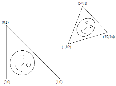
Suppose we have some set. According to the fractal creation algorithm we need to reduce it, rotate and "put on a certain place". The problem is to describe this process using affine transformations, i.e. we need to find the matrix and vector.
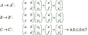
It's easy to prove that it's enough to take 3 points of the initial set (nontrivial) and tranform them into 3 corresponding points of the "reduced" set. This transformation will lead to 6 linear equations, allowing us to find the a,b,c,d,e,f as solution.
Let's show it. Suppose ![]() triangle transformed to
triangle transformed to ![]() triangle.
triangle.
By solving the system of linear equations we will able to get the a,b,c,d,e and f coefficients:
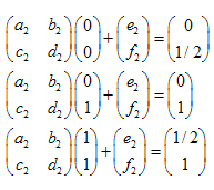
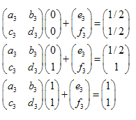
Example:Sierpinski Gasket:
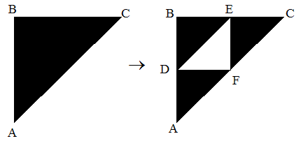
The coordinates of the points are:
- A (0,0)
- B (0,1)
- C (1,1)
- D(0,1/2)
- E (1/2,1)
- F(1/2,1/2)
We have 3 tranformations:
- ABC -> ADF
- ABC -> DBE
- ABC -> FEC
The system of linear equations looks as follows:
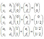
The solutions are: 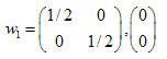 ,
, 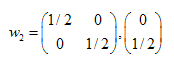 ,
, 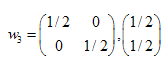
We have found the coefficients of three affine transforms. Furher we will use them for creation of self-similar sets.
3. Creating Fractals Using the Iterated Function Systems
The Iterated Function System (IFS) is a set of affine contractions ![]() where
where![]() - is the "weights". Each of IFS functions is defined by 7 numbers:
- is the "weights". Each of IFS functions is defined by 7 numbers: ![]() , where
, where![]() weights is used when iteration process as a probability of n-th tranformation. It's better to define their values, proportional to contraction:
weights is used when iteration process as a probability of n-th tranformation. It's better to define their values, proportional to contraction: 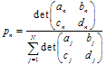 .
.
Let's consider the algorithm of fractal construction using the Iterated Function System (see also Chaos Game).
The first we need is to take some initial point with coordinates ![]() . The next, we choose randomly some of the contractions and plot the point
. The next, we choose randomly some of the contractions and plot the point ![]() . And again, let's choose randomly one of the contractions
. And again, let's choose randomly one of the contractions ![]() and plot
and plot ![]() . Finally we will have the
. Finally we will have the ![]() as a set of points.
as a set of points.
The choice of contraction depend on its "probability". If we repeat the process (for example, to ~30000 points) and plot the resulting set, we will see its structure despite the random process.
Here is an example of Sierpinski Gasket:

Figure 1. The Sierpinski Gasket, generated with IFS coefficients calculated in chapter 2
The code:
//+------------------------------------------------------------------+
//|                                        IFS_Sierpinski_Gasket.mq5 |
//|                        Copyright 2011, MetaQuotes Software Corp. |
//|                                              https://www.mql5.com |
//+------------------------------------------------------------------+
#property copyright "Copyright 2011, MetaQuotes Software Corp."
#property link      "https://www.mql5.com"
#property version   "1.00"

//-- include file with cIntBMP class
#include <cIntBMP.mqh>

//-- Sierpinski Gasket IFS coefficients
//-- (a,b,c,d) matricies
double IFS_a[3] = {0.50,  0.50,  0.50};
double IFS_b[3] = {0.00,  0.00,  0.00};
double IFS_c[3] = {0.00,  0.00,  0.00};
double IFS_d[3] = {0.50,  0.50,  0.50};
//-- (e,f) vectors
double IFS_e[3] = {0.00,  0.00,  0.50};
double IFS_f[3] = {0.00,  0.50,  0.50};
//-- "probabilities" of transforms, multiplied by 1000
double IFS_p[3]={333,333,333};

double Probs[3]; // Probs array - used to choose IFS transforms
cIntBMP bmp;     // cIntBMP class instance
int scale=350;  // scale coefficient
//+------------------------------------------------------------------+
//| Expert initialization function                                   |
//+------------------------------------------------------------------+
int OnInit()
  {
//-- Prepare Probs array
   double m=0;
   for(int i=0; i<ArraySize(IFS_p); i++)
     {
      Probs[i]=IFS_p[i]+m;
      m=m+IFS_p[i];
     }
//-- size of BMP image
   int XSize=500;
   int YSize=400;
//-- create bmp image XSizexYSize with clrSeashell background color
   bmp.Create(XSize,YSize,clrSeashell);
//-- image rectangle
   bmp.DrawRectangle(0,0,XSize-1,YSize-1,clrBlack);

//-- point coordinates (will be used in construction of set)
   double x0=0;
   double y0=0;
   double x,y;
//-- number of points to calculate (more points - detailed image)
   int points=1500000;
//-- calculate set
   for(int i=0; i<points; i++)
     {
      // choose IFS tranform with probabilities, proportional to defined
      double prb=1000*(rand()/32767.0);
      for(int k=0; k<ArraySize(IFS_p); k++)
        {
         if(prb<=Probs[k])
           {
            // affine transformation
            x = IFS_a[k] * x0 + IFS_b[k] * y0 + IFS_e[k];
            y = IFS_c[k] * x0 + IFS_d[k] * y0 + IFS_f[k];
            // update previous coordinates
            x0 = x;
            y0 = y;
            // convert to BMP image coordinates
            // (note the Y axis in cIntBMP)
            int scX = int (MathRound(XSize/2 + (x-0.5)*scale));
            int scY = int (MathRound(YSize/2 + (y-0.5)*scale));
            // if the point coordinates inside the image, draw the dot
            if(scX>=0 && scX<XSize && scY>=0 && scY<YSize) { bmp.DrawDot(scX,scY,clrDarkBlue); }
            break;
           }
        }
     }
//-- save image to file
   bmp.Save("bmpimg",true);
//-- plot image on the chart
   bmp.Show(0,0,"bmpimg","IFS");
//---
   return(0);
  }
//+------------------------------------------------------------------+
//| Expert deinitialization function                                 |
//+------------------------------------------------------------------+
void OnDeinit(const int reason)
  {
//--- delete image from the chart
   ObjectDelete(0,"IFS");
//--- delete file
   bmp.Delete("bmpimg",true);
  }
//+------------------------------------------------------------------+
If we set scale to 1350, increase the number of iterations to 15000000, and change the shift the initial point:
int scX = MathRound(XSize/2 + (x-0.75)*scale);
int scY = MathRound(YSize/2 + (y-0.75)*scale);
we will able to see the zoomed region of the set. One can see (Fig. 2), that it has a self-similar structure:

Figure 2. Zoomed region of Sierpinski Gasket
Let's consider the famous Barnsley's Fern, proposed by Michael Barnsley. It's more complex.

Figure 3. Barnsley's Fern
The code is similar, but in this case we have 4 IFS contractions with different weights.
//+------------------------------------------------------------------+
//|                                                     IFS_fern.mq5 |
//|                        Copyright 2011, MetaQuotes Software Corp. |
//|                                              https://www.mql5.com |
//+------------------------------------------------------------------+
#property copyright "Copyright 2011, MetaQuotes Software Corp."
#property link      "https://www.mql5.com"
#property version   "1.00"
#include <cIntBMP.mqh>
//-- Barnsley Fern IFS coefficients
//-- (a,b,c,d) matricies
double IFS_a[4] = {0.00,  0.85,  0.20,  -0.15};
double IFS_b[4] = {0.00,  0.04, -0.26,   0.28};
double IFS_c[4] = {0.00, -0.04,  0.23,   0.26};
double IFS_d[4] = {0.16,  0.85,  0.22,   0.24};
//-- (e,f) vectors
double IFS_e[4] = {0.00,  0.00,  0.00,   0.00};
double IFS_f[4] = {0.00,  1.60,  1.60,   0.00};
//-- "probabilities" of transforms, multiplied by 1000
double IFS_p[4] = {10,     850,    70,     70};

double Probs[4];
cIntBMP bmp;
int scale=50;
//+------------------------------------------------------------------+
//| Expert initialization function                                   |
//+------------------------------------------------------------------+
int OnInit()
  {
   double m=0;
   for(int i=0; i<ArraySize(IFS_p); i++)
     {
      Probs[i]=IFS_p[i]+m;
      m=m+IFS_p[i];
     }

   int XSize=600;
   int YSize=600;

   bmp.Create(XSize,YSize,clrSeashell);

   bmp.DrawRectangle(0,0,XSize-1,YSize-1,clrBlack);

   double x0=0;
   double y0=0;
   double x,y;

   int points=250000;

   for(int i=0; i<points; i++)
     {
      double prb=1000*(rand()/32767.0);
      for(int k=0; k<ArraySize(IFS_p); k++)
        {
         if(prb<=Probs[k])
           {
            x = IFS_a[k] * x0 + IFS_b[k] * y0 + IFS_e[k];
            y = IFS_c[k] * x0 + IFS_d[k] * y0 + IFS_f[k];
            x0 = x;
            y0 = y;
            int scX = int (MathRound(XSize/2 + (x)*scale));
            int scY = int (MathRound(YSize/2 + (y-5)*scale));
            if(scX>=0 && scX<XSize && scY>=0 && scY<YSize) { bmp.DrawDot(scX,scY,clrForestGreen); }
            break;
           }
        }
     }
   bmp.Save("bmpimg",true);
   bmp.Show(0,0,"bmpimg","IFS");
//---
   return(0);
  }
//+------------------------------------------------------------------+
//| Expert deinitialization function                                 |
//+------------------------------------------------------------------+
void OnDeinit(const int reason)
  {
   ObjectDelete(0,"IFS");
   bmp.Delete("bmpimg",true);
  }
//+------------------------------------------------------------------+
It's remarkable that such complex structure can be defined by only 28 numbers.
If we increase the scale to 150, and set iterations to 1250000 we will see the zoomed fragment:

Figure 4. A fragment of Barnsley's Fern
As you see the algorithm is universal, it allows you to generate different fractal sets.
The next example is Sierpinski Carpet, defined by following IFS coefficients:
//-- Sierpinski Gasket IFS coefficients
double IFS_a[8] = {0.333, 0.333, 0.333, 0.333, 0.333, 0.333, 0.333, 0.333};
double IFS_b[8] = {0.00,  0.00,  0.00,   0.00, 0.00,  0.00,  0.00,   0.00};
double IFS_c[8] = {0.00,  0.00,  0.00,   0.00, 0.00,  0.00,  0.00,   0.00};
double IFS_d[8] = {0.333, 0.333,  0.333,  0.333, 0.333,  0.333,  0.333, 0.333};
double IFS_e[8] = {-0.125, -3.375, -3.375,  3.125, 3.125, -3.375, -0.125, 3.125};
double IFS_f[8] = {6.75, 0.25, 6.75,  0.25, 6.75, 3.5, 0.25, 3.50};
//-- "probabilities", multiplied by 1000
double IFS_p[8]={125,125,125,125,125,125,125,125};

Figure 5. Sierpinski Carpet
In chapter 2 we have considered the algorithm of calculation of coefficients of IFS contractions.
Let's consider how to create the "fractal words". In Russian, the "Fractals" word looks like:

Figure 6. "Fractals" word in Russian
To find the IFS coefficients, we need to solve the corresponding linear systems. The solutions are:
//-- IFS coefficients of the "Fractals" word in Russian
double IFS_a[28]=
  {
   0.00, 0.03,  0.00, 0.09, 0.00, 0.03, -0.00, 0.07, 0.00, 0.07, 0.03,  0.03,  0.03,  0.00,
   0.04, 0.04, -0.00, 0.09, 0.03, 0.03,  0.03, 0.03, 0.03, 0.00, 0.05, -0.00,  0.05,  0.00
  };

double IFS_b[28]=
  {
   -0.11, 0.00, 0.07, 0.00, -0.07, 0.00, -0.11,  0.00, -0.07,  0.00, -0.11,  0.11, 0.00, -0.14,
   -0.12, 0.12,-0.11, 0.00, -0.11, 0.11,  0.00, -0.11,  0.11, -0.11,  0.00, -0.07, 0.00, -0.07
  };

double IFS_c[28]=
  {
   0.12,  0.00,  0.08,  -0.00,  0.08,  0.00,  0.12,  0.00,  0.04,  0.00,  0.12,  -0.12, 0.00,  0.12,
   0.06,  -0.06,  0.10,  0.00,  0.12,  -0.12,  0.00,  0.12,  -0.12,  0.12, 0.00,  0.04,  0.00,  0.12
  };

double IFS_d[28]=
  {
   0.00,  0.05,  0.00,  0.07,  0.00,  0.05,  0.00,  0.07,  0.00,  0.07,  0.00,  0.00,  0.07,  0.00,
   0.00,  0.00,  0.00,  0.07,  0.00,  0.00,  0.07,  0.00,  0.00,  0.00,  0.07,  0.00,  0.07,  0.00
  };

double IFS_e[28]=
  {
   -4.58,  -5.06, -5.16, -4.70, -4.09, -4.35, -3.73, -3.26, -2.76,  -3.26, -2.22, -1.86, -2.04, -0.98,
   -0.46,  -0.76,  0.76,  0.63,  1.78,  2.14,  1.96,  3.11,  3.47,  4.27,  4.60,  4.98,   4.60, 5.24
  };

double IFS_f[28]=
  {
   1.26,  0.89,  1.52,  2.00,  1.52,  0.89,  1.43,  1.96,  1.69,  1.24,  1.43,  1.41,  1.11,  1.43,
   1.79,  1.05,  1.32,  1.96,  1.43,  1.41,  1.11,  1.43,  1.41,  1.43,  1.42,  1.16,  0.71,  1.43
  };

//-- "probabilities", multiplied by 1000
double IFS_p[28]=
  {
   35,  35,  35,  35,  35,  35,  35,  35,  35,  35,  35,  35,  35,  35,
   35,  35,  35,  35,  35,  35,  35,  35,  35,  35,  35,  35,  35,  35
  };
As a result, we will get the following image:

Figure 7. Self-similar word
The full source code can be found in ifs_fractals.mq5.
If we zoom the set, we see the self-similar structure:

Figure 8. Zoomed region of the set
The self-similar sets, based on IFS, can be constructed using the Fractal Designer.
We have covered the topic of creating fractal sets using the Iterated Function Systems. Thanks to the cIntBMP library, the process is very simple. Now it's time to create a class and add some features to make the images better.
You may notice that correct construction of sets driven by probabilites. The difference in probabilities means that set has irregular structure (see weights of Barnsley Fern IFS). This fact can be used for creation of beautiful images. We need to set the color, proportional to the frequency of the point in some neighbourhood.
It can be done using the virtual screen (just an array), if the pixel color will depend on the previous values. Finally, the virtual screen will be rendered into the bmp using the Palette. The bmp image itself can be drawn as a background picture of the chart.
Here is the code of Expert Advisor, based on CIFS class:
//+------------------------------------------------------------------+
//|                                               IFS_Fern_color.mq5 |
//|                        Copyright 2011, MetaQuotes Software Corp. |
//|                                              https://www.mql5.com |
//+------------------------------------------------------------------+
#include <cIntBMP.mqh>
//-- Barnsley Fern IFS coefficients
double IFS_a[4] = {0.00,  0.85,  0.20,  -0.15};
double IFS_b[4] = {0.00,  0.04, -0.26,   0.28};
double IFS_c[4] = {0.00, -0.04,  0.23,   0.26};
double IFS_d[4] = {0.16,  0.85,  0.22,   0.24};
double IFS_e[4] = {0.00,  0.00,  0.00,   0.00};
double IFS_f[4] = {0.00,  1.60,  1.60,   0.00};
double IFS_p[4] = {10,     850,    70,     70};
//-- Palette
uchar Palette[23*3]=
  {
   0x00,0x00,0x00,0x02,0x0A,0x06,0x03,0x11,0x0A,0x0B,0x1E,0x0F,0x0C,0x4C,0x2C,0x1C,0x50,0x28,
   0x2C,0x54,0x24,0x3C,0x58,0x20,0x4C,0x5C,0x1C,0x70,0x98,0x6C,0x38,0xBC,0xB0,0x28,0xCC,0xC8,
   0x4C,0xB0,0x98,0x5C,0xA4,0x84,0xBC,0x68,0x14,0xA8,0x74,0x28,0x84,0x8C,0x54,0x94,0x80,0x40,
   0x87,0x87,0x87,0x9F,0x9F,0x9F,0xC7,0xC7,0xC7,0xDF,0xDF,0xDF,0xFC,0xFC,0xFC
  };
//+------------------------------------------------------------------+
//| CIFS class                                                       |
//+------------------------------------------------------------------+
class CIFS
  {
protected:
   cIntBMP           m_bmp;
   int               m_xsize;
   int               m_ysize;
   uchar             m_virtual_screen[];
   double            m_scale;
   double            m_probs[8];

public:
                    ~CIFS()                          { m_bmp.Delete("bmpimg",true); };
   void              Create(int x_size,int y_size,uchar col);
   void              Render(double scale,bool back);
   void              ShowBMP(bool back);
protected:
   void              VS_Prepare(int x_size,int y_size,uchar col);
   void              VS_Fill(uchar col);
   void              VS_PutPixel(int px,int py,uchar col);
   uchar             VS_GetPixel(int px,int py);
   int               GetPalColor(uchar index);
   int               RGB256(int r,int g,int b) const {return(r+256*g+65536*b);      }
   void              PrepareProbabilities();
   void              RenderIFSToVirtualScreen();
   void              VirtualScreenToBMP();
  };
//+------------------------------------------------------------------+
//| Create method                                                    |
//+------------------------------------------------------------------+
void CIFS::Create(int x_size,int y_size,uchar col)
  {
   m_bmp.Create(x_size,y_size,col);
   VS_Prepare(x_size,y_size,col);
   PrepareProbabilities();
  }
//+------------------------------------------------------------------+
//| Prepares virtual screen                                          |
//+------------------------------------------------------------------+
void CIFS::VS_Prepare(int x_size,int y_size,uchar col)
  {
   m_xsize=x_size;
   m_ysize=y_size;
   ArrayResize(m_virtual_screen,m_xsize*m_ysize);
   VS_Fill(col);
  }
//+------------------------------------------------------------------+
//| Fills the virtual screen with specified color                    |
//+------------------------------------------------------------------+
void CIFS::VS_Fill(uchar col)
  {
   for(int i=0; i<m_xsize*m_ysize; i++) {m_virtual_screen[i]=col;}
  }
//+------------------------------------------------------------------+
//| Returns the color from palette                                   |
//+------------------------------------------------------------------+
int CIFS::GetPalColor(uchar index)
  {
   int ind=index;
   if(ind<=0) {ind=0;}
   if(ind>22) {ind=22;}
   uchar r=Palette[3*(ind)];
   uchar g=Palette[3*(ind)+1];
   uchar b=Palette[3*(ind)+2];
   return(RGB256(r,g,b));
  }
//+------------------------------------------------------------------+
//| Draws a pixel on the virtual screen                              |
//+------------------------------------------------------------------+
void CIFS::VS_PutPixel(int px,int py,uchar col)
  {
   if (px<0) return;
   if (py<0) return;
   if (px>m_xsize) return;
   if (py>m_ysize) return;
    int pos=m_xsize*py+px;
   if(pos>=ArraySize(m_virtual_screen)) return;
   m_virtual_screen[pos]=col;
  }
//+------------------------------------------------------------------+
//| Gets the pixel "color" from the virtual screen                   |
//+------------------------------------------------------------------+
uchar CIFS::VS_GetPixel(int px,int py)
  {
   if (px<0) return(0);
   if (py<0) return(0);
   if (px>m_xsize) return(0);
   if (py>m_ysize) return(0);
    int pos=m_xsize*py+px;
   if(pos>=ArraySize(m_virtual_screen)) return(0);
   return(m_virtual_screen[pos]);
  }
//+------------------------------------------------------------------+
//| Prepare the cumulative probabilities array                       |
//+------------------------------------------------------------------+
void CIFS::PrepareProbabilities()
  {
   double m=0;
   for(int i=0; i<ArraySize(IFS_p); i++)
     {
      m_probs[i]=IFS_p[i]+m;
      m=m+IFS_p[i];
     }
  }
//+------------------------------------------------------------------+
//| Renders the IFS set to the virtual screen                        |
//+------------------------------------------------------------------+
void CIFS::RenderIFSToVirtualScreen()
  {
   double x=0,y=0;
   double x0=0;
   double y0=0;
   uint iterations= uint (MathRound(100000+100*MathPow(m_scale,2)));

   for(uint i=0; i<iterations; i++)
     {
      double prb=1000*(rand()/32767.0);

      for(int k=0; k<ArraySize(IFS_p); k++)
        {
         if(prb<=m_probs[k])
           {
            x = IFS_a[k] * x0 + IFS_b[k] * y0 + IFS_e[k];
            y = IFS_c[k] * x0 + IFS_d[k] * y0 + IFS_f[k];

            int scX = int (MathRound(m_xsize/2 + (x-0)*m_scale));
            int scY = int (MathRound(m_ysize/2 + (y-5)*m_scale));

            if(scX>=0 && scX<m_xsize && scY>=0 && scY<m_ysize)
              {
               uchar c=VS_GetPixel(scX,scY);
               if(c<255) c=c+1;
               VS_PutPixel(scX,scY,c);
              }
            break;
           }
         x0 = x;
         y0 = y;
        }
     }
  }
//+------------------------------------------------------------------+
//| Copies virtual screen to BMP                                     |
//+------------------------------------------------------------------+
void CIFS::VirtualScreenToBMP()
  {
   for(int i=0; i<m_xsize; i++)
     {
      for(int j=0; j<m_ysize; j++)
        {
         uchar colind=VS_GetPixel(i,j);
         int xcol=GetPalColor(colind);
         if(colind==0) xcol=0x00;
         //if(colind==0) xcol=0xFFFFFF;
         m_bmp.DrawDot(i,j,xcol);
        }
     }
  }
//+------------------------------------------------------------------+
//| Shows BMP image on the chart                                     |
//+------------------------------------------------------------------+
void CIFS::ShowBMP(bool back)
  {
   m_bmp.Save("bmpimg",true);
   m_bmp.Show(0,0,"bmpimg","Fern");
   ObjectSetInteger(0,"Fern",OBJPROP_BACK,back);
  }
//+------------------------------------------------------------------+
//| Render method                                                    |
//+------------------------------------------------------------------+
void CIFS::Render(double scale,bool back)
  {
   m_scale=scale;
   VS_Fill(0);
   RenderIFSToVirtualScreen();
   VirtualScreenToBMP();
   ShowBMP(back);
  }

static int gridmode;
CIFS fern;
int currentscale=50;
//+------------------------------------------------------------------+
//| Expert initialization function                                   |
//+------------------------------------------------------------------+
void OnInit()
  {
//-- get grid mode
   gridmode= int (ChartGetInteger(0,CHART_SHOW_GRID,0));
//-- disable grid
   ChartSetInteger(0,CHART_SHOW_GRID,0);
//-- create bmp
   fern.Create(800,800,0x00);
//-- show as backround image
   fern.Render(currentscale,true);
  }
//+------------------------------------------------------------------+
//| Expert deinitialization function                                 |
//+------------------------------------------------------------------+
void OnDeinit(const int r)
  {
//-- restore grid mode
   ChartSetInteger(0,CHART_SHOW_GRID,gridmode);
//-- delete Fern object
   ObjectDelete(0,"Fern");
 }
//+------------------------------------------------------------------+
//| Expert OnChart event handler                                     |
//+------------------------------------------------------------------+
void OnChartEvent(const int id,           // Event identifier
                const long& lparam,   // Event parameter of long type
                const double& dparam, // Event parameter of double type
                const string& sparam  // Event parameter of string type
                )
  {
//--- click on the graphic object
   if(id==CHARTEVENT_OBJECT_CLICK)
     {
      Print("Click event on graphic object with name '"+sparam+"'");
      if(sparam=="Fern")
        {
         // increase scale coefficient (zoom)
         currentscale=int (currentscale*1.1);
         fern.Render(currentscale,true);
        }
     }
  }
//+------------------------------------------------------------------+
The result is:

Figure 9. Barnsley's fern image, created with CIFS class

Figure 10. The zoomed region of Barnsley's Fern

Figure 11. The zoomed region of Barnsley's Fern

Figure 12. The zoomed region of Barnsley's Fern
Do It Yourself
1. There is a lot of IFS fractals in Fractint, for example:
// Binary
double IFS_a[3] = { 0.5,  0.5,  0.0};
double IFS_b[3] = { 0.0,  0.0, -0.5};
double IFS_c[4] = { 0.0,  0.0,  0.5};
double IFS_d[4] = { 0.5,  0.5,  0.5};
double IFS_e[4] = {-2.563477,  2.436544, 4.873085};
double IFS_f[4] = {-0.000000, -0.000003, 7.563492};
double IFS_p[4] = {333, 333, 333};

// Coral
double IFS_a[3] = { 0.307692,  0.307692,  0.000000};
double IFS_b[3] = {-0.531469, -0.076923,  0.54545};
double IFS_c[3] = {-0.461538,  0.153846,  0.692308};
double IFS_d[3] = {-0.293706, -0.447552, -0.195804};
double IFS_e[3] = {5.4019537, -1.295248, -4.893637};
double IFS_f[3] = { 8.655175,  4.152990,  7.269794};
double IFS_p[3] = {400, 150, 450};

// Crystal
double IFS_a[2] = { 0.696970,  0.090909};
double IFS_b[2] = {-0.481061, -0.443182};
double IFS_c[2] = {-0.393939,  0.515152};
double IFS_d[2] = {-0.662879, -0.094697};
double IFS_e[2] = { 2.147003,  4.286558};
double IFS_f[2] = {10.310288,  2.925762};
double IFS_p[2] = {750, 250};

// Dragon
double IFS_a[2] = { 0.824074,  0.088272};
double IFS_b[2] = { 0.281482,  0.520988};
double IFS_c[2] = {-0.212346, -0.463889};
double IFS_d[2] = { 0.864198, -0.377778};
double IFS_e[2] = {-1.882290,  0.785360};
double IFS_f[2] = {-0.110607,  8.095795};
double IFS_p[2] = {780, 220};

// Floor
double IFS_a[3] = { 0,  0.52,  0};
double IFS_b[3] = {-0.5,   0,  0.5};
double IFS_c[3] = { 0.5,   0, -0.5};
double IFS_d[3] = { 0,   0.5,  0};
double IFS_e[3] = {-1.732366, -0.027891,  1.620804};
double IFS_f[3] = { 3.366182,  5.014877,  3.310401};
double IFS_p[3] = {333, 333, 333};

// Koch3
double IFS_a[5] = {0.307692, 0.192308,  0.192308,  0.307692,  0.384615};
double IFS_b[5] = {      0,-0.205882,  0.205882,         0,        0};
double IFS_c[5] = {      0, 0.653846, -0.653846,         0,         0};
double IFS_d[5] = {0.294118, 0.088235,  0.088235,  0.294118, -0.294118};
double IFS_e[5] = {4.119164,-0.688840,  0.688840, -4.136530, -0.007718};
double IFS_f[5] = {1.604278, 5.978916,  5.962514,  1.604278,  2.941176};
double IFS_p[5] = {151, 254, 254, 151, 190};

//Spiral
double IFS_a[3] = { 0.787879, -0.121212,  0.181818};
double IFS_b[3] = {-0.424242,  0.257576, -0.136364};
double IFS_c[3] = { 0.242424,  0.151515,  0.090909};
double IFS_d[3] = { 0.859848,  0.053030,  0.181818};
double IFS_e[3] = { 1.758647,  -6.721654,  6.086107};
double IFS_f[3] = { 1.408065,   1.377236,  1.568035};
double IFS_p[3] = {896, 52, 52};

//Swirl5
double IFS_a[2] = {  0.74545, -0.424242};
double IFS_b[2] = {-0.459091, -0.065152};
double IFS_c[2] = { 0.406061, -0.175758};
double IFS_d[2] = { 0.887121, -0.218182};
double IFS_e[2] = { 1.460279,  3.809567};
double IFS_f[2] = { 0.691072,  6.741476};
double IFS_p[2] = {920, 80};

//Zigzag2
double IFS_a[2] = {-0.632407, -0.036111};
double IFS_b[2] = {-0.614815, 0.444444};
double IFS_c[2] = {-0.545370, 0.210185};
double IFS_d[2] = { 0.659259, 0.037037};
double IFS_e[2] = { 3.840822, 2.071081};
double IFS_f[2] = { 1.282321, 8.330552};
double IFS_p[2] = {888, 112};
Plot these sets. How to find the initial similarity transforms using the IFS coefficients?
2. Create your own fractals sets and calculate their coefficients (chapter 2).
3. Try to play with palette colors (uchar Palette array), extend the palette and add gradient colors.
4. What about the fractal (Hausdorf-Bezikovitch) dimension of Barnsley's Fern? Is there a formula for calculation of fractal dimension using the IFS coefficients*.
5. Add zoom of a certain region, using the information about the mouse click coordinates in OnChartEvent:
void OnChartEvent(const int id,         // Event identifier
                const long& lparam,   // Event parameter of long type
                const double& dparam, // Event parameter of double type
                const string& sparam  // Event parameter of string type
                )
  {
//--- left button click
   if(id==CHARTEVENT_CLICK)
     {
      Print("Coordinates: x=",lparam,"  y=",dparam);
     }
  }
Conclusion
We have considered the algorithm of creation of self-similar sets using the Iterated Function System.
The use of cIntBMP library greatly simplifies the work with graphic images. Besides the DrawDot(x,y,color) method we have used, the cIntBMP class contains many other useful methods. But it's another story.
Translated from Russian by MetaQuotes Ltd.
Original code: https://www.mql5.com/ru/code/328
 DRAW_ARROW
The DRAW_ARROW drawing style plots the arrows (chars).
DRAW_ZIGZAG
The DRAW_ZIGZAG drawing style allow to draw sections using the values of two indicator buffers. It looks like DRAW_SECTION, but it allows to draw vertical sections inside one bar.
VininI Cyber Cyсle [v01]
VininI Cyber Cycle - Identify cyclical movements of price, based on VininI_Cyber Cycle(V2).mq4 by Victor Nicolaev (2009)
Premier Stochastic Oscillator [v01]
Premier Stochastic Oscillator - Double EMA smoothing of stochastic, based on article in TASC by Lee Leibfarth (August 2008)