Every Strategy Tester report ends with a single equity curve, and after enough weeks of work on a system that curve starts to feel like the truth about it. In reality it is one sample. Your rules produced a set of wins and losses, and history dealt them out in one particular order — the order that happened to occur.
That ordering deserves more suspicion than it usually gets. Two strategies with identical trade lists can feel completely different to operate, depending on whether the losses arrived scattered across a decade or packed into one bad quarter. The trade list is the strategy; the ordering is, to a surprising degree, luck.
Monte Carlo simulation is the standard way to separate the two. In this article I want to show how we use one specific variant — trade-order shuffling — in our own USDJPY research, what the resulting numbers changed about our design decisions, and just as important, what this technique cannot tell you.
One backtest is one path
Start with what a backtest result actually is. If your system risks a percentage of equity per trade, the final balance is a product of per-trade growth factors, and multiplication does not care about order. Shuffle the trades and the final balance lands in the same place.
The path is a different matter. Maximum drawdown, the length of losing streaks, the depth of the worst month — all of these depend on which trades happened to land next to each other. A 5% historical drawdown may hide orderings of the same trades that would have produced 12%.
This matters even more once the system reacts to its own path. Any rule of the form "stop trading after losing X% from the peak" breaks the symmetry: under one ordering the rule never fires, under another it fires in year two and everything after that point never happens. The equity curve in your report shows one of these worlds. Your risk lives in the others.
Turning one path into a distribution
So the useful question is not "what was the maximum drawdown?" but something closer to: across the orderings this trade population could plausibly have arrived in, how often does the outcome cross the line where I would have to stop?
Order-shuffling Monte Carlo answers exactly that question, and the procedure is short. Take the trades from the backtest. Randomize their order and rebuild the equity path. Repeat thousands of times, then count how many paths cross whatever threshold matters to you.
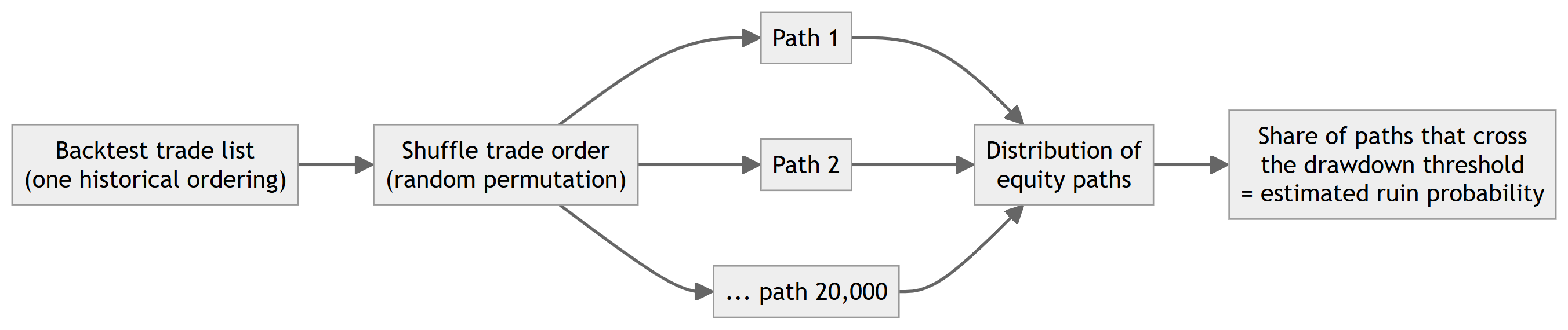
What comes out is not a prettier equity curve. It is a single uncomfortable number: an estimate of ruin probability, given your trade population and your stopping rule.
What we measured on our own system
Some context for the concrete example. Our USDJPY portfolio system was validated on roughly 19 years of real tick data (2007–2026, real-tick modeling, 98% history quality, with about 0.7 pips of total trading cost included). The system carries a hard rule we call the permanent stop: if equity falls 18% from its peak, it stops trading and does not restart. That threshold is a real system action, not a reporting line, so "how often do we reach 18%?" decides whether the system survives at all.
We estimated that probability by shuffling the backtest trade sequence 20,000 times and counting the paths that touched the 18% line, separately for each of the three risk settings the system exposes. The figures below are simulation and backtest results, not live performance.
| Risk setting | 19-year CAGR (backtest) | Max drawdown (historical path) | Reached the 18% stop (Monte Carlo, 20,000 runs) |
|---|---|---|---|
| Default | 12.7% | 5.2% | 1.35% |
| Medium | 16.0% | 6.4% | 7.75% |
| High | 2.7% | 19.0% | 17.9% |
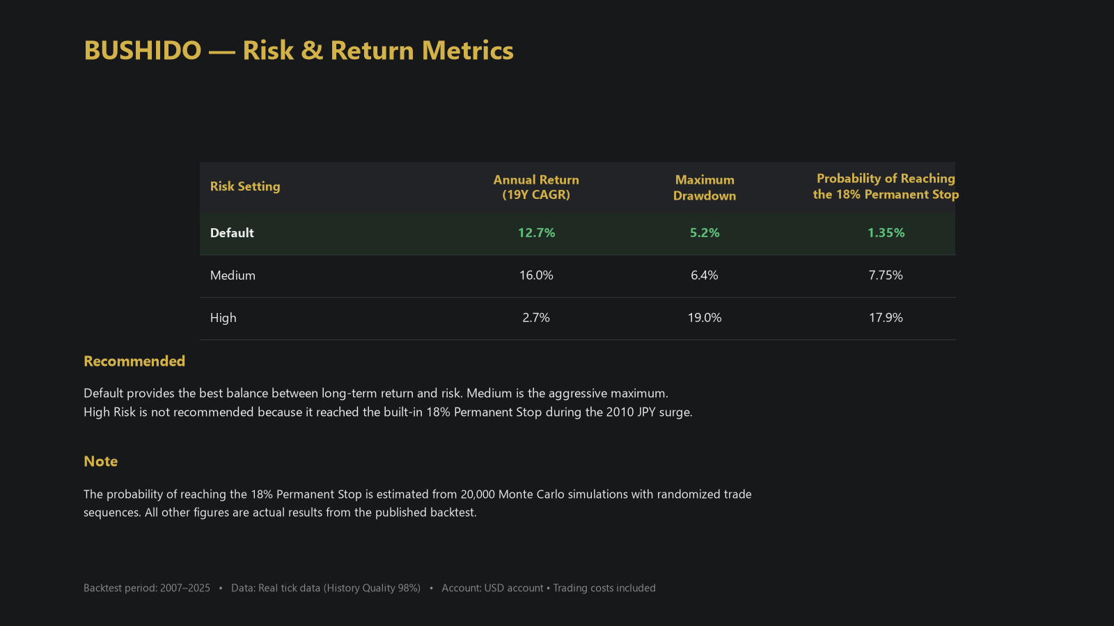
The Default row is worth reading slowly. A 5.2% historical drawdown sounds comfortable against an 18% stop — more than three times the headroom. The Monte Carlo estimate adds the nuance the single path cannot show: even with that much room, about 1.35% of orderings still find their way to the stop. Roughly 270 of the 20,000 simulated paths ended a system that, on the historical path, never came close to ending.
The High row taught us the most. Raising risk lifted the drawdowns to where nearly one in five shuffled paths (17.9%) crossed the stop. On the actual historical path it did cross: during the yen surge of 2010, the High setting reached the 18% threshold, the permanent stop fired, and compounding ended right there. Nineteen years later, the backtest CAGR of that setting stands at 2.7% — below the conservative Default's 12.7%. Not because the trades were worse. The system simply did not survive to compound them; the historical ordering happened to fall inside that 17.9%.
That table is the reason the conservative setting is the recommended one and the high-risk setting explicitly is not. Past a certain point, more risk did not buy more long-term return. It bought a meaningful chance of not being in the market for the second half of the test.
What the number changes in practice
Before running these simulations, our design discussions sounded like most people's: "max drawdown was 5%, that seems fine." Afterward they sounded different — "this setting fails in 1.35% of orderings; is that acceptable for a system someone may run with real money?"
The second form is better for a few reasons. A drawdown statistic is a point estimate from one path, and as shown above, the path is partly luck; a threshold-crossing probability uses the same data to describe the whole population of plausible paths. It also maps onto a real decision. No account has a rule that triggers at "maximum drawdown" — real accounts have a line, enforced by the system, the broker, or the trader's own nerves, beyond which trading stops. Estimating the probability of hitting that specific line answers the question that actually matters.
There is a quieter benefit as well. To run the simulation at all, you must first write down where your stop really is, and deciding that number honestly is half the value of the exercise. If you would realistically abandon a strategy at 15% down, testing survival against 30% is self-deception.
What order-shuffling cannot tell you
Now the honest half of the article. A shuffle test rests on the assumption that trades are independent and could have arrived in any order. Markets do not fully cooperate with that assumption.
Real losses cluster. A strategy that suffers in a specific market regime — a volatility spike, a long directionless range — will concentrate its losing trades in those calendar stretches. Shuffling scatters those losses across the timeline, which can make the tail look thinner than it is. In that sense, order-shuffling is often an optimistic estimator. Treat its ruin probability as a lower bound, not a guarantee.
A partial remedy for the clustering problem exists. Instead of shuffling individual events, you can shuffle contiguous blocks of results — whole weeks or months — so that short-range clustering survives inside each block. Block-based resampling keeps more of the market's serial character and usually produces fatter, more honest tails. It is not a complete fix either: the block length becomes a new assumption of its own, and nothing inside the procedure recovers dependence that operates on scales longer than the blocks. A reasonable way to use the two variants is as a bracket — the plain shuffle marks the optimistic end of the range, a block shuffle moves you a step toward realism, and the truth about the tail sits somewhere between them.
A shuffle test also cannot detect overfitting. A curve-fit strategy produces a beautiful trade list, and 20,000 permutations of a beautiful trade list all look beautiful. The simulation inherits every bias present in its input.
For both reasons we treat Monte Carlo as one gate among several. In our research pipeline it sits alongside chronological out-of-sample splits and a final untouched holdout period — methods that test precisely the things shuffling cannot, such as regime dependence and fitting to the past.
Count events, not report rows
One technical detail decides whether your simulation means anything: the unit you shuffle.
Tester reports are organized in rows, and rows are not decisions. If a strategy scales out of one position in three steps, the report shows three profitable rows — but there was one trade idea, one entry decision, one market event. Shuffle those three rows as independent draws and you have manufactured diversification that never existed, which quietly shrinks your simulated drawdowns.
The principle we follow is to resample at the level of independent events. Everything that stands or falls with a single decision gets collapsed into one return before any shuffling starts. It is a mundane data-preparation step, and it changes tail estimates more than most modeling choices do.
In MetaTrader 5 terms, the deal history is the wrong granularity by default. A single position usually produces several deal rows — the entry, possibly partial closes, the final exit — and the report may carry separate rows for swaps and commission adjustments. Group the deals by position identifier first. If your strategy scales into or out of positions, go one step further and group the positions that belong to one trading decision. The right grouping rule depends on how your EA actually behaves, which is exactly why no generic tool can perform this step for you — and why skipping it quietly biases every number that comes out afterward.
Trying this on your own system
You do not need special tooling to apply any of this to an Expert Advisor you are testing. The whole procedure fits in a spreadsheet or a short script in any language.
Export the deal history from your Strategy Tester report. Collapse the rows into per-event returns, merging partial fills and scale-outs that belong to one decision, and express each event as a percentage change so the results generalize beyond one starting balance. Then shuffle the sequence with a proper random generator, rebuild the equity path, apply your own stopping line — the drawdown level where you would genuinely quit — and record whether the path crossed it. Repeat a few thousand times; the crossing frequency is your estimate.
Two practical notes from doing this on our own reports. Use enough runs for the tail you are trying to measure — if the true probability is near 1%, a few hundred simulations will estimate it mostly by noise, while 20,000 runs put a few hundred paths in that tail and the estimate starts to mean something. And resist the urge to soften the stopping line after seeing the results. Moving the threshold until the number looks acceptable is the same mistake as optimizing a parameter until the backtest looks good; it just happens one layer higher.
There is simple arithmetic behind the run-count advice. The standard error of an estimated probability p over N independent runs is roughly the square root of p(1−p)/N. At p = 1% and N = 500 runs, that error is about 0.44 percentage points — your "1%" could easily read as 0.5% or as 2%, which is the difference between a comfortable design and a questionable one. At N = 20,000 the same error shrinks to about 0.07 percentage points, and the estimate becomes stable enough to compare settings against each other. (These are arithmetic properties of the estimator, not trading results.) Runs are cheap; a spreadsheet-level implementation completes tens of thousands of them in seconds, so there is rarely a good reason to economize here.
One last reporting habit worth adopting: whenever you write a ruin-probability number down — for yourself or for anyone else — record the run count and the stopping line next to it. "1.35% at an 18% stop over 20,000 runs" is a reproducible statement. "About 1%" is not, and six months later you will not remember which threshold it referred to.
Closing thoughts
The next time an equity curve impresses you — your own or a vendor's — it is worth asking what fraction of its reshuffled siblings would have survived the stopping rule you actually intend to use. The answer is sometimes reassuring and sometimes not, but either way it is information a single backtest cannot provide, and it costs an evening of scripting to obtain.
Origin-U Project is an independent quantitative foreign exchange research project based in Japan. The concepts discussed in this article are implemented in Bushido, a commercial USDJPY portfolio EA developed by Origin-U Project.
All performance figures in this article are backtest or Monte Carlo simulation results based on historical data. Past results do not guarantee future performance.
Origin-U Research Notes — Part 5 of 10
← Previous: Why We Chose Not to Use Martingale or Grid Systems | Next: What Makes a Robust Forex Strategy: Judging the Process, Not the Chart →
日本語版: モンテカルロ・シミュレーションでトレーディングシステムを評価する
Full series
- Building a Multi-Strategy Portfolio EA for USDJPY: What 86 Tested Hypotheses Taught Us
- Why Diversification Matters in Algorithmic Trading
- Risk Management Before Profit: Designing the Loss Side of a Trading System First
- Why We Chose Not to Use Martingale or Grid Systems
- Using Monte Carlo Simulation to Evaluate Trading Systems
- What Makes a Robust Forex Strategy: Judging the Process, Not the Chart
- The Difference Between Backtesting and Forward Testing
- How We Evaluate Trading Ideas Before Implementation
- Designing Low Drawdown Trading Systems: Drawdown as an Input, Not an Outcome
- Lessons Learned from Long-Term USDJPY Research: What 20 Years of Tick Data Taught Us