Basic math behind Forex trading

Introduction

I am a developer of automatic strategies and software with over 5 years of experience. In this article, I will open the veil of secrecy to those just starting to trade in Forex or on any other exchange. Besides, I will try to answer the most popular trading questions.

I hope, the article will be useful for both beginners and experienced traders. Also, note that this is purely my vision based on actual experience and research.

Some of the mentioned robots and indicators can be found in my products. But this is only a small part. I have developed a wide variety of robots that apply a plethora of strategies. I will try to show how the described approach allows gaining insight into the true nature of the market and which strategies are worth paying attention to.

Why is it so challenging to find entry and exit points?

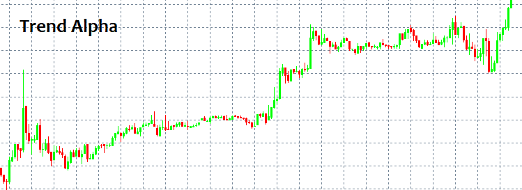
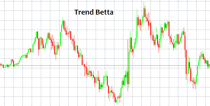
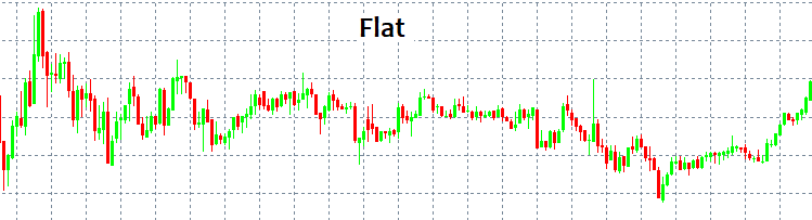
If you know where to enter and exit the market, you probably don't need to know anything else. Unfortunately, the issue of entry/exit points is an elusive one. At first glance, you can always identify a pattern and follow it for a while. But how to detect it without sophisticated tools and indicators? The simplest and always recurring patterns are TREND and FLAT. Trend is a long-term movement in one direction, while Flat implies more frequent reversals.

These patterns can be easily detected since a human eye can find them without any indicators. The main issue here is that we can see a pattern only after it has been triggered. Moreover, no one can guarantee there has been any pattern at all. No pattern can save your deposit from destruction regardless of a strategy. I will try to provide possible reasons for this using the language of math.

Market mechanisms and levels

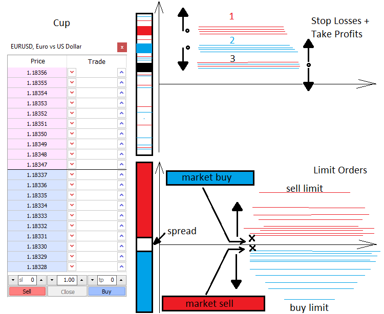
Let me tell you a little about pricing and powers that make the market price move. There are two forces in the market — Market and Limit. Similarly, there are two types of orders — market and limit ones. Limit buyers and sellers fill in the market depth, while market ones take it apart. The market depth is basically a vertical price scale indicating those willing to buy or sell something. There is always a gap between limit sellers and buyers. This gap is called a spread. Spread is a distance between the best buy and sell prices measured in the number of minimal price movements. Buyers want to buy at the cheapest price, while sellers want to sell at the highest price. Therefore, limit orders of buyers are always located at the bottom, while orders of sellers are always located at the top. Marker buyers and sellers enter the market depth and two orders (limit and market ones) are linked. The market movement occurs when a limit order is triggered.

When an active market order appears, it usually has Stop Loss and Take Profit. Similar to limit orders, these stop levels are scattered all around the market forming price acceleration or reversal levels. Everything depends on the amount and type of stop levels, as well as deal volume. Knowing these levels, we can say where the price may accelerate or reverse.

Limit orders can also form fluctuations and clusters that are hard to pass through. They usually appear at important price points, such as an opening of a day or a week. When discussing level-based trading, traders usually mean using limit order levels. All this can be briefly displayed as follows.

Mathematical description of the market

What we see in the MetaTrader window is a discrete function of the t argument, where t is time. The function is discrete because the number of ticks is finite. In the current case, ticks are points containing nothing in between. Ticks are the smallest elements of possible price discretization, larger elements are bars, M1, M5, M15 candles, etc. The market features both the element of random and patterns. The patterns can be of various scales and duration. However, the market is for the most part a probabilistic, chaotic and almost unpredictable environment. To understand the market, one should view it through the concepts of the probability theory. Discretization is needed to introduce the concepts of probability and probability density. 

To introduce the concept of the expected payoff, we first need to consider the terms 'event' and 'exhaustive events':

• C1 event — Profit, it is equal to tp
• C2 event — Loss, it is equal to sl
• P1 — C1 event probability
• P2 — C2 event probability

С1 and С2 events form an exhaustive group of antithetic events (i.e. one of these events occurs in any case). Therefore, the sum of these probabilities is equal to one P2(tp,sl) +  P2(tp,sl) = 1. This equation may turn out to be handy later.

While testing an EA or a manual strategy with a random opening, as well as random StopLoss and TakeProfit, we still get one non-random result and the expected payoff equal to "-(Spread)", which would mean "0", if we could set the spread to zero. This suggests that we always get the zero expected payoff on the random market regardless of stop levels. On the non-random market, we always get a profit or loss provided that the market features related patterns. We can reach the same conclusions by assuming that the expected payoff (Tick[0].Bid - Tick[1].Bid) is also equal to zero. These are fairly simple conclusions that can be reached in many ways. 

• M=P1*tp-P2*sl= P1*tp-(1- P1)*sl  — for any market
  
  
• P1*tp-P2*sl= 0 — for the chaotic market
  

This is the main chaotic market equation describing the expected payoff of a chaotic order opening and closing using stop levels. After solving the last equation, we get all the probabilities we are interested in, both for the complete randomness and the opposite case, provided that we know stop values. 

The equation provided here is meant only for the simplest case that can be generalized for any strategy. This is exactly what I am going to do now to achieve a complete understanding of what constitutes the final expected payoff we need to make non-zero. Also, let's introduce the concept of profit factor and write the appropriate equations.

Assume that our strategy involves closing both by stop levels and some other signals. To do this, I will introduce the С3, С4 event space, in which the first event is closing by stop levels, while the second one is closing by signals. They also form a complete group of antithetic events, so we can use the analogy to write:

M=P3*M3+P4*M4=P3*M3+(1-P3)*M4, where  M3=P1*tp-(1- P1)*sl, while  M4=Sum(P0[i]*pr[i]) - Sum(P01[j]*ls[j]);  Sum( P0[i] )+  Sum( P01[j] ) =1

• M3 — expected payoff when closing by a stop order.
• M4  — expected payoff when closing by a signal.
• P1 , P2  — probabilities of stop levels activation provided that one of the stop levels is triggered in any case.
  
• P0[i]   — probability of closing a deal with the profit of pr[i] provided that it has not triggered stop levels. i  — closing option number
  
• P01[j]  — probability of closing a deal with the loss of ls[j]  provided that it has not triggered stop levels. j  — closing option number
  

In other words, we have two antithetic events. Their outcomes form another two independent event spaces where we also define the full group. However, the P1, P2, P0[i] and P01[j] probabilities are conditional now, while P3 and P4 are the probabilities of hypotheses. The conditional probability is a probability of an event when a hypothesis occurs. Everything is in strict accordance with the total probability formula (Bayes' formula). I strongly recommend studying it thoroughly to grasp the matter. For a completely chaotic trading, M=0.

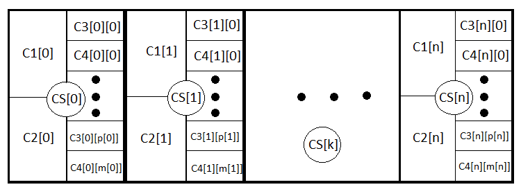
Now the equation has become much clearer and broader, as it considers closing both by stop levels and signals. We can follow this analogy even further and write the general equation for any strategy that takes into account even dynamic stop levels. This is what I am going to do. Let's introduce N new events forming a complete group meaning opening deals with similar StopLoss and TakeProfit. CS[1] .. CS[2] .. CS[3] ....... CS[N] . Similarly, PS[1] + PS[2] + PS[3] + ....... +PS[N] = 1.

M = PS[1]*MS[1]+PS[2]*MS[2]+ ... + PS[k]*MS[k] ... +PS[N]*MS[N] , MS[k] = P3[k]*M3[k]+(1- P3[k])*M4[k],  M3[k] =  P1[k] *tp[k] -(1- P1[k] )*sl[k], M4[k] =  Sum(i)(P0[i][k]*pr[i][k]) - Sum(j)(P01[j][k] *ls[j][k] );  Sum(i)( P0[i][k]  )+  Sum(j)( P01[j][k]  ) =1.

• PS[k]  — probability of setting k th stop level option.
  
• MS[k]  —   expected payoff of closed deals with k th stop levels.
  
• M3[k]  — expected payoff when closing by a stop order with k th stop levels.
• M4[k]  — expected payoff when closing by a signal with k th stop levels.
• P1[k] , P2[k]  — probabilities of stop levels activation provided that one of the stop levels is triggered in any case.
  
• P0[i][k]  — probability of closing a deal with pr[i][k]  profit, according to a signal with k th stop levels. i  — closing option number
  
• P01[j][k]  — probability of closing a deal with ls[j][k]  loss, according to a signal with k th stop levels.  j  — closing option number

Like in the previous (more simple) equations, M=0 in case of chaotic trading and absence of a spread. The most you can do is change the strategy but if it contains no rational basis, you will simply change the balance of these variables and still get 0. In order to break this unwanted equilibrium, we need to know the probability of the market movement in any direction within any fixed movement segment in points or the expected price movement payoff within a certain period of time. Entry/exit points are selected depending on that. If you manage to find them, then you will have a profitable strategy.

Now let's create the profit factor equation. PF = Profit/Loss. The profit factor is the ratio of profit to loss. If the number exceeds 1, the strategy is profitable, otherwise, it is not. This can be redefined using the expected payoff. PrF=Mp/Ml. This means the ratio of the expected net profit payoff to the expected net loss. Let's write their equations.

• Mp = PS[1]*MSp[1]+PS[2]*MSp[2]+ ... + PS[k]*MSp[k] ... +PS[N]*MSp[N] , MSp[k] = P3[k]*M3p[k]+(1- P3[k])*M4p[k] ,  M3p[k] =  P1[k] *tp[k], M4p[k] =  Sum(i)(P0[i][k]*pr[i][k])
  
  
• Ml = PS[1]*MSl[1]+PS[2]*MSl[2]+ ... + PS[k]*MSl[k] ... +PS[N]*MSl[N] , MSl[k] = P3[k]*M3l[k]+(1- P3[k])*M4l[k] ,  M3l[k] =   (1- P1[k] )*sl[k], M4l[k] =  Sum(j)(P01[j][k]*ls[j][k])
  

Sum(i)( P0[i][k] ) +  Sum(j)( P01[j][k]  ) =1.

• MSp[k]  —   expected payoff of closed deals with k th stop levels.
• MSl[k]  —   expected payoff of closed deals with k th stop levels. 
  
• M3p[k]  — expected payoff when closing by a stop order with k th stop levels.
• M4p[k]  — expected payoff when closing by a signal with k th stop levels.
• M3l[k]  — expected loss when closing by a stop order with k th stop levels.
• M4l[k]  — expected loss when closing by a signal with k th stop levels.

For a deeper understanding, I will depict all nested events:

In fact, these are the same equations, although the first one lacks the part related to loss, while the second one lacks the part related to profit. In case of chaotic trading, PrF = 1 provided that the spread is equal to zero again. M and PrF  are two values that are quite sufficient to evaluate the strategy from all sides.

In particular, there is an ability to evaluate the trend or flat nature of a certain instrument using the same probability theory and combinatorics. Besides, it is also possible to find some differences from randomness using the probability distribution densities.

I will build a random value distribution probability density graph for a discretized price at a fixed H step in points. Let's assume that if the price moves H in any direction, then a step has been taken. The X axis is to display a random value in the form of a vertical price chart movement measured in the number of steps. In this case, n steps are imperative as this is the only way to evaluate the overall price movement.

• n  — total number of steps (constant value)
• d  — number of steps for price drop
• u  — number of steps for price increase
• s  — total upward movement in steps

After defining these values, calculate u and d:

To provide the total "s" steps upwards (the value can be negative meaning downward steps), a certain number of up and down steps should be provided: "u", "d". The final "s" up or down movement depends on all steps in total:

n=u+d;

s=u-d;

This is a system of two equations. Solving it yields u and d:

u=(s+n)/2, d=n-u.

However, not all "s" values are suitable for a certain "n" value. The step between possible s values is always equal to 2. This is done in order to provide "u" and "d" with natural values since they are to be used for combinatorics, or rather, for calculating combinations. If these numbers are fractional, then we cannot calculate the factorial, which is the cornerstone of all combinatorics. Below are all possible scenarios for 18 steps. The graph shows how extensive the event options are.

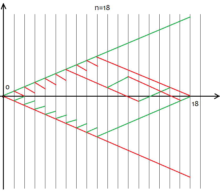
It is easy to define that the number of options comprises 2^n for the whole variety of pricing options since there are only two possible movement directions after each step – up or down. There is no need to try to grasp each of these options, as it is impossible. Instead we just simply need to know that we have n unique cells, of which u and d should be up and down, respectively. The options having the same u and d ultimately provide the same s. In order to calculate the total number of options providing the same "s", we can use the combination equation from the combinatorics С=n!/(u!*(n-u)!), as well as the equivalent equation С=n!/(d!*(n-d)!). In case of different u and d, we obtain the same value of C. Since the combinations can be made both by ascending and descending segments, this inevitably leads to déjà vu. So what segments should we use to form combinations? The answer is any, as these combinations are equivalent despite their differences. I will try to prove this below using a MathCad 15-based application.

Now that we have determined the number of combinations for each scenario, we can determine the probability of a particular combination (or event, whatever you like). P =  С/(2^n). This value can be calculated for all "s", and the sum of these probabilities is always equal to 1, since one of these options will happen anyway. Based on this probability array, we are able to build the probability density graph relative to the "s" random value considering that s step is 2. In this case, the density at a particular step can be obtained simply by dividing the probability by the s step size, i.e. by 2. The reason for this is that we are unable to build a continuous function for discrete values. This density remains relevant half a step to the left and right, i.e. by 1. It helps us find the nodes and allows for numerical integration. For negative "s" values, I will simply mirror the graph relative to the probability density axis. For even n values, numbering of nodes starts from 0, for odd ones it starts from 1. In case of even n values, we cannot provide odd s values, while in case of odd n values, we cannot provide even s values. The calculation application screenshot below clarifies this:

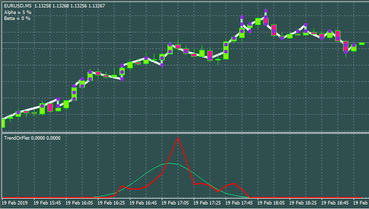
It lists everything we need. The application is attached below so that you are able to play around with the parameters. One of the most popular questions is how to define whether the current market situation is trend or flat-based. I have come up with my own equations for quantifying the trend or flat nature of an instrument. I have divided trends into Alpha and Beta ones. Alpha means a tendency to either buy or sell, while Beta is just a tendency to continue the movement without a clearly defined prevalence of buyers or sellers. Finally, flat means a tendency to get back to the initial price.

The definitions of trend and flat vary greatly among traders. I am trying to give a more rigid definition to all these phenomena, since even a basic understanding of these matters and means of their quantification allows applying many strategies previously considered dead or too simplistic. Here are these main equations: 

K=Integral(p*|x|)

or

K=Summ(P[i]*|s[i]|)

The first option is for a continuous random variable, while the second one is for a discrete one. I have made the discrete value continuous for more clarity, thus using the first equation. The integral spans from minus to plus infinity. This is the equilibrium or trend ratio. After calculating it for a random value, we obtain an equilibrium point to be used to compare the real distribution of quotes with the reference one. If Кp > K, the market can be considered trending. If Кp < K, the market is flat.

We can calculate the maximum value of the ratio. It is equal to KMax=1*Max(|x|) or KMax=1*Max(|s[i]|). We can also calculate the minimum value of the ratio. It is equal to KMin=1*Min(|x|) = 0 or KMin=1*Min(|s[i]|) = 0. The KMid midpoint, minimum and maximum are all that is needed to evaluate trend or flat nature of the analyzed area in percentage.

if ( K >= KMid ) KTrendPercent=((K-KMid)/(KMax-KMid))*100  else  KFletPercent=((KMid-K)/KMid)*100.  

But this is still not enough to fully characterize the situation. Here is where the second ratio T=Integral(p*x),  T=Summ(P[i]*s[i]) comes to the rescue. It essentially shows the expected payoff of the number of upward steps and is at the same time an indicator of the alpha trend. Tp > 0 means a buy trend, while Tp < 0 means a sell trend, i.e. T=0 is for the random walk. 

Let's find the maximum and minimum value of the ratio:  TMax=1*Max(x) or TMax=1*Max(s[i]), the minimum one in absolute value is equal to the maximum one, but it is simply negative  TMin= - TMax. If we measure the alpha trend percentage from 100 to -100, we may write equations for calculating the value similar to the previous one:

APercent=( T /TMax)*100.

If the percentage is positive, the trend is bullish, if it is negative, the trend is bearish.  The cases may be mixed. There may be an alpha flat and alpha trend but not trend and flat simultaneously. Below is a graphical illustration of the above statements and examples of constructed density graphs for various number of steps.

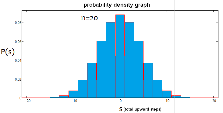
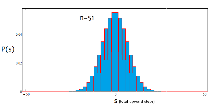
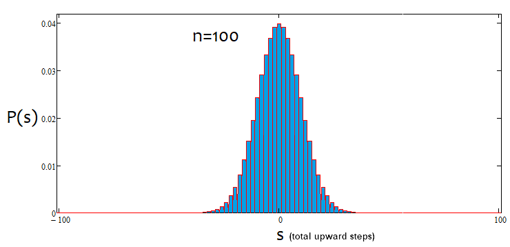
As we can see, with an increase in the number of steps, the graph becomes narrower and higher. For each number of steps, the corresponding alpha and beta values are different, just like the distribution itself. When changing the number of steps, the reference distribution should be recalculated.

All these equations can be applied to build automated trading systems. These algorithms can also be used to develop indicators. Some traders have already implemented these things in their EAs. I am sure of one thing: it is better to apply this analysis rather than avoid it. Those familiar with math will immediately come up with some new ideas on how to apply it. Those who are not will have to make more efforts.

Writing a simple indicator

Here I am going to transform my simple mathematical research into an indicator detecting market entry points and serving as a basis for writing EAs. I will develop the indicator in MQL5. However, the code is to be adapted for porting to MQL4 for the greatest possible extent. Generally, I try to use the simplest possible methods resorting to OOP only if a code becomes unnecessarily cumbersome and unreadable. However, this can be avoided in 90% of cases. Unnecessarily colorful panels, buttons and a plethora of data displayed on a chart only hinder the visual perception. Instead, I always try to do with as little visual tools as possible.

Let's start from the indicator inputs.

input uint BarsI=990;//Bars TO Analyse ( start calc. & drawing )
input uint StepsMemoryI=2000;//Steps In Memory
input uint StepsI=40;//Formula Steps
input uint StepPoints=30;//Step Value
input bool bDrawE=true;//Draw Steps

When the indicator is loaded, we are able to carry out the initial calculation of a certain number of steps using certain last candles as a basis. We will also need the buffer to store data about our last steps. The new data is to replace the old one. Its size is to be limited. The same size is to be used to draw steps on the chart. We should specify the number of steps, for which we are to build distribution and calculate the necessary values. Then we should inform the system of the step size in points and whether we need visualization of steps. Steps are to be visualized by drawing on the chart.

I have selected the indicator style in a separate window displaying the neutral distribution and the current situation. There are two lines, although it would be good to have the third one. Unfortunately, the indicators capabilities do not imply drawing in a separate and main windows, so I have had to resort to drawing.

I always use the following little trick to be able to access bar data like in MQL4:

//variable to be moved in MQL5
double Close[];
double Open[];
double High[];
double Low[];
long Volume[];
datetime Time[];
double Bid;
double Ask;
double Point=_Point;
int Bars=1000;
MqlTick TickAlphaPsi;

void DimensionAllMQL5Values()//set the necessary array size
   {
   ArrayResize(Close,BarsI,0);
   ArrayResize(Open,BarsI,0);   
   ArrayResize(Time,BarsI,0);
   ArrayResize(High,BarsI,0);
   ArrayResize(Low,BarsI,0);
   ArrayResize(Volume,BarsI,0);
   }

void CalcAllMQL5Values()//recalculate all arrays
   {
   ArraySetAsSeries(Close,false);                        
   ArraySetAsSeries(Open,false);                           
   ArraySetAsSeries(High,false);                        
   ArraySetAsSeries(Low,false);                              
   ArraySetAsSeries(Volume,false);
   ArraySetAsSeries(Time,false);                                                            
   if( Bars >= int(BarsI) ) 
      {
      CopyClose(_Symbol,_Period,0,BarsI,Close);
      CopyOpen(_Symbol,_Period,0,BarsI,Open);   
      CopyHigh(_Symbol,_Period,0,BarsI,High);
      CopyLow(_Symbol,_Period,0,BarsI,Low);
      CopyTickVolume(_Symbol,_Period,0,BarsI,Volume); 
      CopyTime(_Symbol,_Period,0,BarsI,Time);      
      }
   ArraySetAsSeries(Close,true);
   ArraySetAsSeries(Open,true);
   ArraySetAsSeries(High,true);                        
   ArraySetAsSeries(Low,true);
   ArraySetAsSeries(Volume,true);                                                                                                
   ArraySetAsSeries(Time,true);
   SymbolInfoTick(Symbol(),TickAlphaPsi);
   Bid=TickAlphaPsi.bid;
   Ask=TickAlphaPsi.ask;
   }
////////////////////////////////////////////////////////////

Now the code is made compatible with MQL4 as much as possible and we are able to turn it into an MQL4 analogue quickly and easily.

To describe the steps, we first need to describe the nodes.

struct Target//structure for storing node data
   {
   double Price0;//node price
   datetime Time0;//node price
   bool Direction;//direction of a step ending at the current node
   bool bActive;//whether the node is active
   };
   
double StartTick;//initial tick price
Target Targets[];//destination point ticks (points located from the previous one by StepPoints)

Additionally, we will need a point to count the next step from. The node stores data about itself and the step that ended on it, as well as the boolean component that indicates whether the node is active. Only when the entire memory of the node array is filled with real nodes, the real distribution is calculated since it is calculated by steps. No steps — no calculation.

Further on, we need to have the ability to update the status of steps at each tick and carry out an approximate calculation by bars when initializing the indicator.

bool UpdatePoints(double Price00,datetime Time00)//update the node array and return 'true' in case of a new node
   {
   if ( MathAbs(Price00-StartTick)/Point >= StepPoints )//if the step size reaches the required one, write it and 
shift the array back
      {
      for(int i=ArraySize(Targets)-1;i>0;i--)//first move everything back
         {
         Targets[i]=Targets[i-1];
         }
      //after that, generate a new node  
      Targets[0].bActive=true;
      Targets[0].Time0=Time00;
      Targets[0].Price0=Price00;
      Targets[0].Direction= Price00 > StartTick ? true : false;
      //finally, redefine the initial tick to track the next node
      StartTick=Price00;
      return true;
      }
   else return false;
   }

void StartCalculations()//approximate initial calculations (by bar closing prices)
   {
   for(int j=int(BarsI)-2;j>0;j--) 
      {
      UpdatePoints(Close[j],Time[j]);
      }  
   }

Next, describe the methods and variables necessary to calculate all neutral line parameters. Its ordinate represents the probability of a particular combination or outcome. I do not like to call this the normal distribution since the normal distribution is a continuous quantity, while I build the graph of a discrete value. Besides, the normal distribution is a probability density rather than probability as in the case of the indicator. It is more convenient to build a probability graph, rather than its density.

int S[];//array of final upward steps
int U[];//array of upward steps
int D[];//array of downward steps
double P[];//array of particular outcome probabilities

double KBettaMid;//neutral Betta ratio value
double KBettaMax;//maximum Betta ratio value
//minimum Betta = 0, there is no point in setting it
double KAlphaMax;//maximum Alpha ratio value
double KAlphaMin;//minimum Alpha ratio value
//average Alpha = 0, there is no point in setting it

int CalcNumSteps(int Steps0)//calculate the number of steps
   {
   if ( Steps0/2.0-MathFloor(Steps0/2.0) == 0 ) return int(Steps0/2.0);
   else return int((Steps0-1)/2.0);
   }

void ReadyArrays(int Size0,int Steps0)//prepare the arrays
   {
   int Size=CalcNumSteps(Steps0);
   ArrayResize(S,Size);
   ArrayResize(U,Size);
   ArrayResize(D,Size);
   ArrayResize(P,Size);
   ArrayFill(S,0,ArraySize(S),0);//clear
   ArrayFill(U,0,ArraySize(U),0);
   ArrayFill(D,0,ArraySize(D),0);
   ArrayFill(P,0,ArraySize(P),0.0);
   }

void CalculateAllArrays(int Size0,int Steps0)//calculate all arrays
   {
   ReadyArrays(Size0,Steps0);
   double CT=CombTotal(Steps0);//number of combinations
   for(int i=0;i<ArraySize(S);i++)
      {
      S[i]=Steps0/2.0-MathFloor(Steps0/2.0) == 0 ? i*2 : i*2+1 ;
      U[i]=int((S[i]+Steps0)/2.0);
      D[i]=Steps0-U[i];
      P[i]=C(Steps0,U[i])/CT;
      }
   }

void CalculateBettaNeutral()//calculate all Alpha and Betta ratios
   {
   KBettaMid=0.0;
   if ( S[0]==0 )
      {
      for(int i=0;i<ArraySize(S);i++)
         {
         KBettaMid+=MathAbs(S[i])*P[i];
         }
      for(int i=1;i<ArraySize(S);i++)
         {
         KBettaMid+=MathAbs(-S[i])*P[i];
         }
      }
   else
      {
      for(int i=0;i<ArraySize(S);i++)
         {
         KBettaMid+=MathAbs(S[i])*P[i];
         }
      for(int i=0;i<ArraySize(S);i++)
         {
         KBettaMid+=MathAbs(-S[i])*P[i];
         }
      }
   KBettaMax=S[ArraySize(S)-1];
   KAlphaMax=S[ArraySize(S)-1];
   KAlphaMin=-KAlphaMax;
   }
   
double Factorial(int n)//factorial of n value
   {
   double Rez=1.0;
   for(int i=1;i<=n;i++)
      {
      Rez*=double(i);
      }
   return Rez;
   }
   
double C(int n,int k)//combinations from n by k
   {
   return Factorial(n)/(Factorial(k)*Factorial(n-k));
   }
   
double CombTotal(int n)//number of combinations in total
   {
   return MathPow(2.0,n);
   }

All these functions should be called in the right place. All functions here are intended either for calculating the values of arrays, or they implement some auxiliary mathematical functions, except for the first two. They are called during initialization along with the calculation of the neutral distribution, and used to set the size of the arrays.

Next, create the code block for calculating the real distribution and its main parameters in the same way.

double AlphaPercent;//alpha trend percentage
double BettaPercent;//betta trend percentage
int ActionsTotal;//total number of unique cases in the Array of steps considering the number of steps for checking the option
int Np[];//number of actual profitable outcomes of a specific case
int Nm[];//number of actual losing outcomes of a specific case
double Pp[];//probability of a specific profitable step
double Pm[];//probability of a specific losing step
int Sm[];//number of losing steps

void ReadyMainArrays()//prepare the main arrays
   {
   if ( S[0]==0 )
      {
      ArrayResize(Np,ArraySize(S));
      ArrayResize(Nm,ArraySize(S)-1);
      ArrayResize(Pp,ArraySize(S));
      ArrayResize(Pm,ArraySize(S)-1);      
      ArrayResize(Sm,ArraySize(S)-1);
      for(int i=0;i<ArraySize(Sm);i++)
         {
         Sm[i]=-S[i+1];
         }
      ArrayFill(Np,0,ArraySize(Np),0);//clear
      ArrayFill(Nm,0,ArraySize(Nm),0);
      ArrayFill(Pp,0,ArraySize(Pp),0);
      ArrayFill(Pm,0,ArraySize(Pm),0);      
      }
   else
      {
      ArrayResize(Np,ArraySize(S));
      ArrayResize(Nm,ArraySize(S));
      ArrayResize(Pp,ArraySize(S));
      ArrayResize(Pm,ArraySize(S));      
      ArrayResize(Sm,ArraySize(S));
      for(int i=0;i<ArraySize(Sm);i++)
         {
         Sm[i]=-S[i];
         }
      ArrayFill(Np,0,ArraySize(Np),0);//clear
      ArrayFill(Nm,0,ArraySize(Nm),0);
      ArrayFill(Pp,0,ArraySize(Pp),0);
      ArrayFill(Pm,0,ArraySize(Pm),0);            
      }   
   }

void CalculateActionsTotal(int Size0,int Steps0)//total number of possible outcomes made up of the array of steps
   {
   ActionsTotal=(Size0-1)-(Steps0-1);
   }

bool CalculateMainArrays(int Steps0)//count the main arrays
   {
   int U0;//upward steps
   int D0;//downward steps
   int S0;//total number of upward steps
   if ( Targets[ArraySize(Targets)-1].bActive )
      {
      ArrayFill(Np,0,ArraySize(Np),0);//clear
      ArrayFill(Nm,0,ArraySize(Nm),0);
      ArrayFill(Pp,0,ArraySize(Pp),0);
      ArrayFill(Pm,0,ArraySize(Pm),0);      
      for(int i=1;i<=ActionsTotal;i++)
         {
         U0=0;
         D0=0;
         S0=0;
         for(int j=0;j<Steps0;j++)
            {
            if ( Targets[ArraySize(Targets)-1-i-j].Direction ) U0++;
            else D0++;
            }
         S0=U0-D0;
         
         for(int k=0;k<ArraySize(S);k++)
            {
            if ( S[k] == S0 )
               {
               Np[k]++;
               break;
               }
            }
         for(int k=0;k<ArraySize(Sm);k++)
            {
            if ( Sm[k] == S0 )
               {
               Nm[k]++;
               break;
               }
            }
         }
         
      for(int k=0;k<ArraySize(S);k++)
         {
         Pp[k]=Np[k]/double(ActionsTotal);
         }
      for(int k=0;k<ArraySize(Sm);k++)
         {
         Pm[k]=Nm[k]/double(ActionsTotal);
         }         
         
      AlphaPercent=0.0;
      BettaPercent=0.0;
      for(int k=0;k<ArraySize(S);k++)
         {
         AlphaPercent+=S[k]*Pp[k];
         BettaPercent+=MathAbs(S[k])*Pp[k];
         }
      for(int k=0;k<ArraySize(Sm);k++)
         {
         AlphaPercent+=Sm[k]*Pm[k];
         BettaPercent+=MathAbs(Sm[k])*Pm[k];
         }
      AlphaPercent= (AlphaPercent/KAlphaMax)*100;
      BettaPercent= (BettaPercent-KBettaMid) >= 0.0 ? ((BettaPercent-KBettaMid)/(KBettaMax-KBettaMid))*100 : ((BettaPercent-KBettaMid)/KBettaMid)*100;
      
      Comment(StringFormat("Alpha = %.f %%\nBetta = %.f %%",AlphaPercent,BettaPercent));//display these numbers on the screen
      return true;
      }
   else return false;
   }

Here all is simple but there are much more arrays since the graph is not always mirrored relative to the vertical axis. To achieve this, we need additional arrays and variables, but the general logic is simple: calculate the number of specific case outcomes and divide it by the total number of all outcomes. This is how we get all probabilities (ordinates) and the corresponding abscissas. I am not going to delve into each loop and variable. All these complexities are needed to avoid issues with moving values to the buffers. Here everything is almost the same: define the size of arrays and count them. Next, calculate the alpha and beta trend percentages and display them in the upper left corner of the screen.

It remains to define what and where to call.

int OnInit()
  {
   //--- indicator buffers mapping
   SetIndexBuffer(0,NeutralBuffer,INDICATOR_DATA);
   SetIndexBuffer(1,CurrentBuffer,INDICATOR_DATA);
   CleanAll();
   DimensionAllMQL5Values();
   CalcAllMQL5Values();
   StartTick=Close[BarsI-1];
   ArrayResize(Targets,StepsMemoryI);//maximum number of nodes
   CalculateAllArrays(StepsMemoryI,StepsI);
   CalculateBettaNeutral();
   StartCalculations();
   ReadyMainArrays();
   CalculateActionsTotal(StepsMemoryI,StepsI);
   return(INIT_SUCCEEDED);
  }
//+------------------------------------------------------------------+
//| Custom indicator iteration function                              |
//+------------------------------------------------------------------+
int OnCalculate(const int rates_total,
                const int prev_calculated,
                const datetime &time[],
                const double &open[],
                const double &high[],
                const double &low[],
                const double &close[],
                const long &tick_volume[],
                const long &volume[],
                const int &spread[])
  {
  CalcAllMQL5Values();
  
  if ( UpdatePoints(Close[0],TimeCurrent()) )
     {
     if ( CalculateMainArrays(StepsI) )
        {
        if ( bDrawE ) RedrawAll();
        }
     }
      
  int iterator=rates_total-(ArraySize(Sm)+ArraySize(S))-1;
  for(int i=0;i<ArraySize(Sm);i++)
     {
     iterator++;
     NeutralBuffer[iterator]=P[ArraySize(S)-1-i];
     CurrentBuffer[iterator]=Pm[ArraySize(Sm)-1-i];
     }
  for(int i=0;i<ArraySize(S);i++)
     {
     iterator++;
     NeutralBuffer[iterator]=P[i];
     CurrentBuffer[iterator]=Pp[i];
     }

   return(rates_total);
  }

CurrentBuffer and NeutralBuffer are used here as buffers. For more clarity, I have introduced the display on the nearest candles to the market. Each probability is on a separate bar. This allowed us to get rid of unnecessary complications. Simply zoom the chart in and out to see everything. The CleanAll() and RedrawAll() functions are not shown here. They can be commented out, and everything will work fine without rendering. Also, I have not included the drawing block here. You can find it in the attachment. There is nothing notable there. The indicator is also attached below in two versions — for MetaTrader 4 and MetaTrader 5.

This will look as follows.

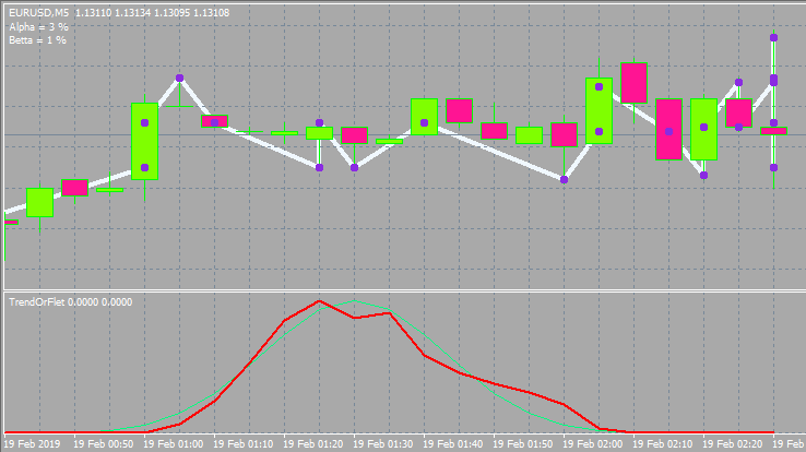
Below is the option with other inputs and window style.

Review of the most interesting strategies

I have developed and seen plenty of strategies. In my humble experience, the most notable things happen when using a grid or martingale or both. Strictly speaking, the expected payoff of both martingale and grid is 0. Do not be fooled by upward-going charts since one day you will get a huge loss. There are working grids and they can be found in the market. They work fairly well and even show the profit factor of 3-6. This is quite a high value. Moreover, they remain stable on any currency pair. But it is not easy to come up with filters that will allow you to win. The method described above allows you to sort these signals out. The grid requires a trend, while the direction is not important. 

Martingale and grid are the examples of the most simple and popular strategies. However, not everyone is able to apply them in the proper way. Self-adapting Expert Advisors are a bit more complex. They are able to adapt to anything be it flat, trend or any other patterns. They usually involve taking a certain piece of the market to look for patterns and trade a short period of time in the hope that the pattern will remain for some time.

A separate group is formed by exotic systems with mysterious, unconventional algorithms attempting to profit on the chaotic nature of the market. Such systems are based on pure math and able to make a profit on any instrument and time period. The profit is not big but stable. I have been dealing with such systems lately. This group also involves brute force-based robots. The brute force can be performed using additional software. In the next article, I will show my version of such a program.

The top niche is occupied by robots based on neural networks and similar software. These robots show very different results and feature the highest level of sophistication since the neural network is a prototype of AI. If a neural network has been properly developed and trained, it is able to show the highest efficiency unmatched by any other strategy.

As for arbitration, in my opinion, its possibilities are now almost equal to zero. I have the appropriate EAs yielding no results.

Is it worth the hassle?

Someone trades on markets out of excitement, someone looks for easy and quick money, while someone wants to study market processes via equations and theories. Besides, there are traders simply having no other choice since there is no way back for them. I mostly belong to the latter category. With all my knowledge and experience, I currently don't have a profitable stable account. I have EAs showing good test runs but everything is not as easy as it seems ).

Those striving to get rich quickly will most probably face the opposite result. After all, the market is not created for a common trader to win. It has quite the opposite objective. However, if you are brave enough to venture into the topic, then make sure you have plenty of time and patience. The result will not be quick. If you have no programming skills, then you have practically no chance at all. I've seen a lot of pseudo traders bragging about some results after having traded 20-30 deals. In my case, after I develop a decent EA, it may work one or two years but then it inevitably fails...In many cases, it does not work from the start.

Of course, there is such thing as manual trading, but I believe it is more akin to art. All in all, it is possible to make money on the market, but you will spend a lot of time. Personally, I don't think it is worth it. From the mathematical perspective, the market is just a boring two-dimensional curve. I certainly do not want to look at candles my entire life ).

Does the Grail exist and where to look for it?

I believe that the Grail is more than possible. I have relatively simple EAs proving it. Unfortunately, their expected payoff barely covers the spread. I think almost every developer has strategies confirming this. The Market has plenty of robots that can be called Grails in all respects. But making money with such systems is extremely difficult as you need to fight for each pip, as well as enable spread return and partnership programs. Grails featuring considerable profits and low deposit loads are rare.

If you want to develop a Grail on your own, then it is better to look towards neural networks. They have much potential in terms of profit. Of course, you can try to combine various exotic approaches and brute force, bit I recommend delving into neural networks right away.

Oddly enough, the answer to the questions of whether a Grail exists and where to look for one is quite simple and obvious to me after tons of EAs I have developed.

Tips for common traders

All traders want three things:

• Achieve a positive expected payoff
• Increase profit in case of a profitable position
• Reduce loss in case of a losing position

The first point is the most important here. If you have a profitable strategy (regardless of whether it is manual or algorithmic), you will always want to intervene. This should not be allowed. Situations, in which profitable deals are less numerous than losing ones, exert a considerable psychological impact ruining a trading system. Most importantly, do not rush to win back your losses when you are in the red. Otherwise, you may find yourself with even more losses. Remember about an expected payoff. It does not matter what the current position's equity loss is. What really matters is the total number of positions and the profit/loss ratio.

The next important thing is a lot size you apply in your trading. If you are currently in profit, make sure to gradually reduce the lot. Otherwise, increase it. However, it should be increased only up to a certain threshold value. This is a forward and reverse martingale. If you think carefully, you can develop your own EA based purely on lot variations. This will no longer be a grid or martingale, but something more complex and safe. Besides, such an EA may work on all currency pairs throughout the history of quotes. This principle works even in a chaotic market, and it does not matter where and how you enter. With proper use, you will compensate for all spreads and commissions, and with masterful use, you will come out with a profit even if you enter the market at a random point and in a random direction.

To reduce losses and increase profits, try to buy on a negative half-wave and sell on a positive half-wave. A half-way usually indicates the previous activity of buyers or sellers in the current market area, which in turn means that some of them have been market ones, while open positions will close sooner or later pushing the price in the opposite direction. That is why the market has a wave structure. We can see these waves everywhere. A purchase is followed by a selling and vice versa. Also close your positions using the same criterion.

Conclusion

Everyone's perspective is subjective. In the end, it all depends on you, one way or another. Despite all the disadvantages and wasted time, everyone wants to create their own super system and reap the fruits of their determination. Otherwise, I do not see the point of delving into Forex trading at all. This activity somehow remains attractive to many traders including myself. Everyone knows how this feeling is called, but it will sound childish. Therefore, I will not name it to avoid trolling. )