How Long Is the Trend?

MetaTrader 5 — Tester | 25 May 2017, 10:03

23 536

Introduction

Determining market conditions at different time periods is the fundamental principle of exchange trading. The success of a trader depends on how accurate their price forecast is. A number of articles have already been written on the topic, e.g. "Several Ways of Finding a Trend in MQL5", which describes the methods for determining the trend market, with relevant indicators and Expert Advisors. One of my previous articles "Comparative Analysis of 10 Trend Strategies " is also devoted to the trend, in which trend following strategies were developed and tested. In this article, we'll also choose several methods for determining the trend, aiming to establish the duration of trend relative to the flat market. It is generally accepted that the trend to flat ratio is 30% to 70%. We will check this.

Defining the task

Let's determine the tasks and conditions for our research.

To select methods for determining trend and flat markets for subsequent quantitative and qualitative analysis. This requires only the systems that show both market conditions. Ideally, they should have built-in quality indicators such as trend power or a clear definition of the sideways trend.
To be able to determine and evaluate the ratio on different time periods and on different single- and multi-commodity markets, be it currency, stock or futures markets.
To develop a tool useful to the reader enabling an independent research in user-specific conditions.
To perform a comparative analysis based on data obtained under different conditions; to search for correlation.

Implementation

1. Selecting the methods for determining the trend.

1.1. Let's start the research with ADX, the classic trend power indicator. We will estimate trend or flat zones using the level of TrendLevel. Let's assume that the trend exists if the main line rises above this level. Fig. 1 shows an example of determining Trend Zone and Flat Zone using this method. The market state will be calculated for the number of candlesticks where the ADX value is higher than TrendLevel from the given sample.

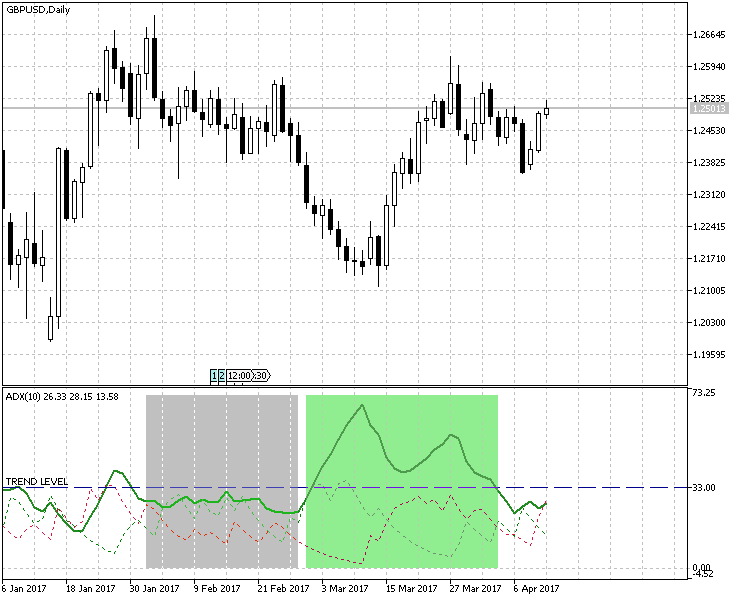
Fig.1 Using ADX to determine the trend/flat zone

1.2. Next, let's consider Trend Power and Direction Indicator, choosing, for our purposes, only one Bollinger Indicator and reducing the displayed number of colors to two (red and green). Fig. 2 clearly shows strong market trends, where candlesticks are marked with specified colors.

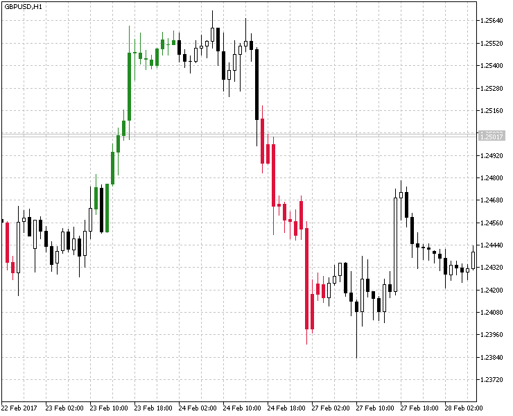
Fig.2 Using Bollinger Bands to determine the trend/flat zones.

1.3. In third place, we'll consider the Percentage of Trend, which we've also modified by removing the second period and adding the color indication for the trend. The result of applying this indicator is shown in Fig.3

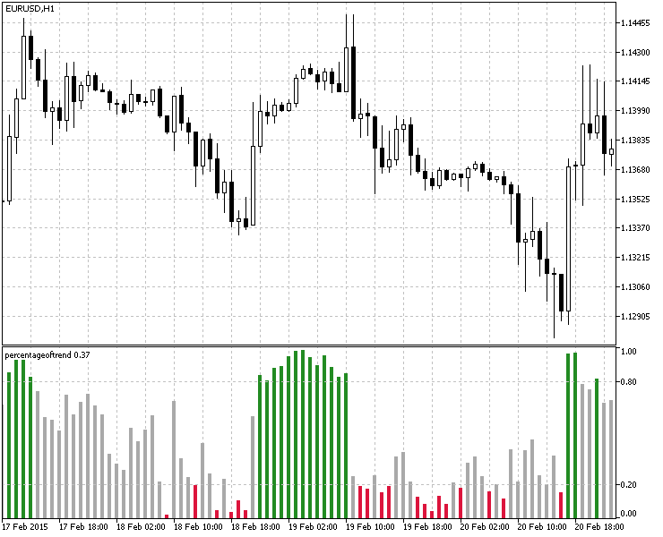
Fig.3 Using Percentage of Trend to determine the trend/flat zones.

1.4. Another way to determine the trend/flat zone is the RSIFilter. For easier calculation, the RSI indicator is displayed as a histogram with vertical columns that show indicator values entering the preset overbought/oversold zones. Here, the original indicator has been changed, too: the flat state is not displayed and the buffer for histogram height value in this market condition equals zero. This is done for more convenient determination of a trend (in which case the buffer value is equal to one). An example of the indicator is shown in Fig.4

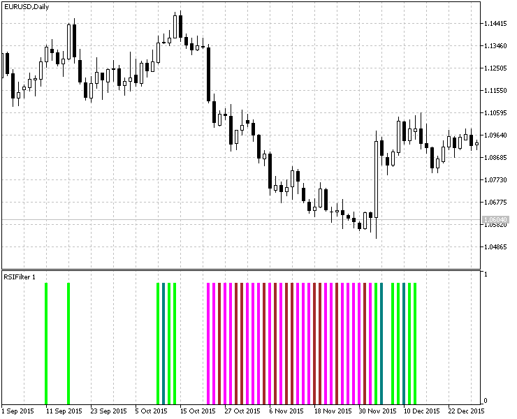
Fig. 4 Using RSIFilter to determine the trend/flat zone.

1.5. Finally, we will consider the method from the article "Several Ways of Finding a Trend in MQL5" — the method of identifying trend/flat states using the ZigZagTrendDetector Indicator. There are no changes in this case. Its implementation is shown in Fig.5

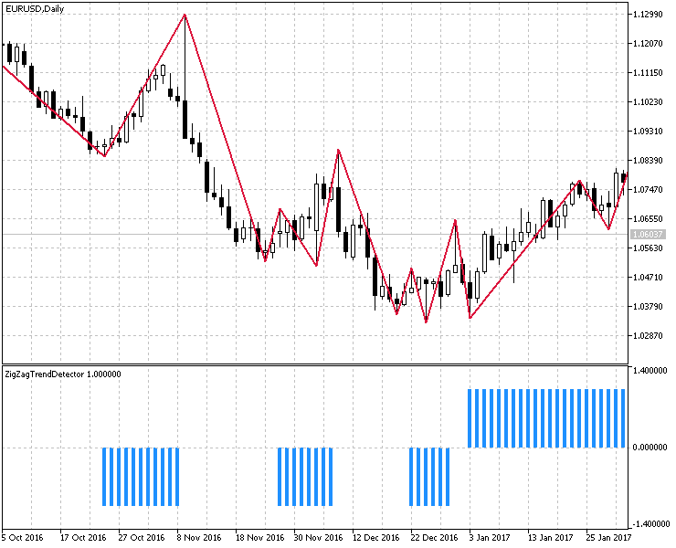
Fig. 5 Determination of trend/flat zones using ZigZagTrendDetector.

2. Development and implementation of a tool for calculating market conditions. Displaying the results.

The result for each method of determining the trend/flat zones will be shown as a summary table for several timeframes. For clarity of the presentation, I used the EasyAndFastGUI library based on the Graphical Interfaces article series. A special class CTrendCountUI was developed to visualize the results. For better representation, Fig. 6 shows the original template used to record all the calculations.

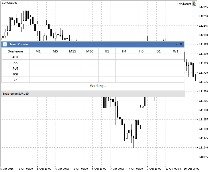
Fig.6 The template displaying the calculation of test results.

As you can see in the screenshot, the first column shows methods for calculating the trend, the first line shows calculation for a multi-timeframe option. To save space and preserve readability, I leave out the full implementation of the interface, giving only the function that configures and visualizes the template presented above:

//+------------------------------------------------------------------+
//| Output and configuration of the information panel                |
//+------------------------------------------------------------------+
void SetInfoPanel()
  {
//---

   UI.CreateMainPanel("Trend Counter");
   UI.CreateStatusBar(1,25);
   UI.m_status_bar.ValueToItem(0,"Enabled on "+Symbol());
   UI.CreateCanvasTable();
//---

   UI.m_canvas_table.SetValue(0,0,"Value");
   UI.m_canvas_table.SetValue(0,1,"ADX");
   UI.m_canvas_table.SetValue(0,2,"BB");
   UI.m_canvas_table.SetValue(0,3,"PoT");
   UI.m_canvas_table.SetValue(0,4,"RSI");
   UI.m_canvas_table.SetValue(0,5,"ZZ");
//---

   UI.m_canvas_table.SetValue(1,0,"M1");
   UI.m_canvas_table.SetValue(2,0,"M5");
   UI.m_canvas_table.SetValue(3,0,"M15");
   UI.m_canvas_table.SetValue(4,0,"M30");
   UI.m_canvas_table.SetValue(5,0,"H1");
   UI.m_canvas_table.SetValue(6,0,"H4");
   UI.m_canvas_table.SetValue(7,0,"H6");
   UI.m_canvas_table.SetValue(8,0,"D1");
   UI.m_canvas_table.SetValue(9,0,"W1");

   UI.m_canvas_table.UpdateTable(true);
   UI.CreateLabel("Working...");
  }

The next step is to create calculation algorithms for the above calculation methods. Most of implementation options are similar so we will analyze only one of them. Let's dwell on the calculation.

We start with the first described method - ADX, the GetADXCount() function.

//+------------------------------------------------------------------+
//| The function for calculating market conditions using ADX         |
//+------------------------------------------------------------------+
bool GetADXCount()
  {
//--- Блок 1
   double adx[],result[],count;
   int to_copy,bars;
   int tf_size=ArraySize(Ind_Timeframe);
   ArrayResize(Ind_Handle,tf_size);
   ArrayResize(result,tf_size);
   ArrayInitialize(adx,0.0);
   ArrayInitialize(result,0.0);
   ArraySetAsSeries(adx,true);
//---

   for(int i=0;i<tf_size;i++)
     {
      count=0;
      Ind_Handle[i]=iADX(Symbol(),Ind_Timeframe[i],InpInd_ADXPeriod);
      if(Ind_Handle[i]==INVALID_HANDLE)
        {
         Print(" Failed to get the indicator handle");
         return(false);
        }
      //--- Block 2

      bars=Bars(Symbol(),Ind_Timeframe[i]);
      to_copy=(bars<NumCandles)?bars:NumCandles;
      //---

      if(CopyBuffer(Ind_Handle[i],0,0,to_copy,adx)<=0)
         return(false);
      //--- Block 3

      for(int j=0;j<to_copy;j++)
        {
         if(adx[j]>TrendLevel)
            count++;
        }
      result[i]=(count/to_copy)*100;
      IndicatorRelease(Ind_Handle[i]);
     }
//--- Block 4

   for(int i=1;i<=tf_size;i++)
      UI.m_canvas_table.SetValue(i,1,DoubleToString(result[i-1],2));
   UI.m_canvas_table.UpdateTable(true);
   return(true);
  }

Let's consider the blocks of code from the listing above.

Block 1. Initialization of variables and arrays, their reduction to the number of timeframes used for testing.
Block 2. A sample of a certain number of candlesticks, for testing and obtaining the percentage result. Note that on higher timeframes or instruments with a small history, there may be not enough bars for a given sample, so you need to determine the history depth and, if necessary, adjust the volume of data requested.
Block 3. For the ADX indicator, we will increment the counter when its value for the current bar goes above the TrendLevel.
Block 4. We add the test results to a table prepared earlier in the SetInfoPanel() function.

Subsequently, only the Block 3 (the counting conditions) will be altered.

The GetColorBBCount() function.

for(int j=0;j<to_copy;j++)
        {
         if(bb[j])
            count++;
        }
result[i]=(count/to_copy)*100;

The non-zero value of the selected indicator buffer means that the current candlestick in the sample belongs to trend. Otherwise this is a flat period.

The GetPoTCount() function.

The parameters of the 'Percentage of Trend' indicator are the following:

//--- Percentage of Trend parameters

input int                  InpPeriodPoT=20;
input double               UpTrendLevel=0.8;
input double               DnTrendLevel=0.2;

Therefore, an indication of trend existence is an indicator value going beyond the UpTrendLevel and DnTrendLevel levels. Accordingly, the calculation will look like the following:

 for(int j=0;j<to_copy;j++)
        {
         if(pot[j]>=UpTrendLevel || pot[j]<=DnTrendLevel)
            count++;
        }
 result[i]=(count/to_copy)*100;

The GetRSICount() function.

Since the function is represented as a histogram, in which 1 indicates the existence of a trend and 0 shows its absence, the condition is identical to GetColorBBCount():

 for(int j=0;j<to_copy;j++)
        {
         if(rsi[j])
            count++;
        }
 result[i]=(count/to_copy)*100;

The GetZZCount() function.

Similar to the previous one, the same histogram form of the indicator.

 for(int j=0;j<to_copy;j++)
        {
         if(zz[j])
            count++;
        }
 result[i]=(count/to_copy)*100;

The GetAverage() function.

Calculates the overall result for all methods and timeframes.

//+------------------------------------------------------------------+
//| The function of calculating the mean value for all data          |
//+------------------------------------------------------------------+
string GetAverage(double &arr[])
  {
   double sum=0.0;
   int size=ArraySize(arr);
   for(int i=0;i<size;i++)
      sum+=arr[i];
   sum/=size;
   return(DoubleToString(sum,2));
  }
//+------------------------------------------------------------------+

As a result, data calculation and output have the following compact representation:

//+------------------------------------------------------------------+
//| Expert initialization function                                   |
//+------------------------------------------------------------------+
int OnInit()
  {
   SetInfoPanel();
   if(GetADXCount() && 
      GetColorBBCount() && 
      GetPoTCount() && 
      GetRSICount() && 
      GetZZCount()
      )
      UI.m_label1.LabelText("Done. Result for "+IntegerToString(NumCandles)+" bars. Average Trend Time - "+GetAverage(avr_result)+"%");
   else
     {
      UI.m_label1.LabelText("Error");
     }
//---
   return(INIT_SUCCEEDED);
  }

Testing

For testing, it was decided to use several various instruments in order to maximize the range of research conditions:

Currency pairs - EURUSD, USDCHF, USDJPY, GBPUSD;
Futures (GOLD-6.17);
Stock market (#MCD);

On all timeframes, testing will take place on a sample of 2,000 bars. Here are the testing parameters, which are identical for all symbols.

//+------------------------------------------------------------------+
//| Expert input parameters                                          |
//+------------------------------------------------------------------+

input int                  NumCandles=2000;              //Number of analyzed candles
//---- ADX parameters
input string               com1="";                      //---- ADX parameters
input int                  InpInd_ADXPeriod=14;          //ADX Period
input double               TrendLevel=20.0;
//--- ColorBBCandles parameters
input string               com2="";                      //---- ColorBBCandles parameters
input int                  BandsPeriod=20;               // BB averaging period
input double               BandsDeviation=1.0;           // Deviation
input ENUM_MA_METHOD       MA_Method_=MODE_SMA;          // Indicator averaging method
input Applied_price_       IPC=PRICE_CLOSE_;             // Price constant
//--- Percentage of Trend parameters
input string               com3="";                      //---- Percentage of Trend parameters
input int                  InpPeriodPoT=20;
input double               UpTrendLevel=0.7;
input double               DnTrendLevel=0.3;
//--- RSIFilter parameters
input string               com4="";                      //---- RSIFilter parameters
input uint                 RSIPeriod=10;                 // Indicator period
input ENUM_APPLIED_PRICE   RSIPrice=PRICE_CLOSE;         // Price
input uint                 HighLevel=60;                 // Overbought level
input uint                 LowLevel=40;                  // Oversold level
//--- ZigZagTrendDetector parameters
input string               com5="";                      //---- ZigZagTrendDetector parameters
input int                  ExtDepth=5;
input int                  ExtDeviation= 5;
input int                  ExtBackstep = 3;

1. Testing of currency pairs.

The results of testing on four currency pairs reveal the prevailing average value equal to 60% of the time in the trend state. At the same time, there are no significant differences observed from using different methods and timeframes.

Fig. 7. Four currency pairs, testing results.

2. Testing on futures.

The results of testing on futures showed that higher timeframes inhibit values that stand out of the overall tendency. This is because initially we've set a sample series of 2,000 bars, but on D1 and W1 there is not enough history for that, so the calculation is based on the maximum available history.

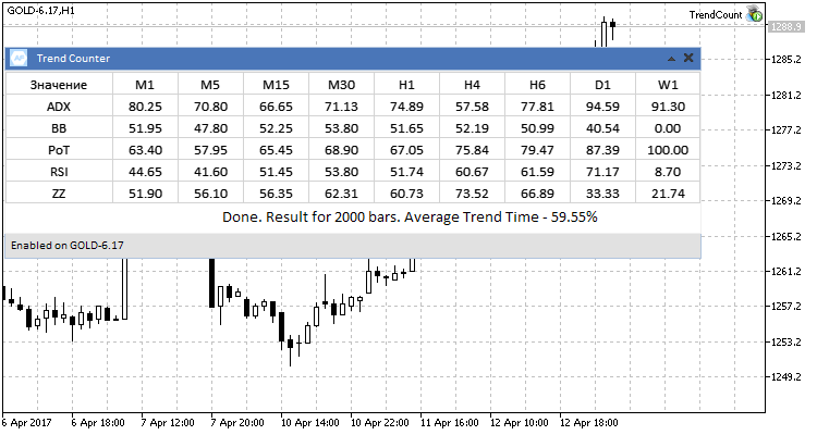
Fig.7 Testing results for futures GOLD-6.17.

3. Testing on stocks.

Here, too, there is a general tendency, already observed on the above symbols.

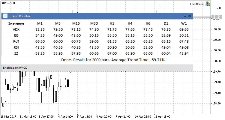
Fig.8 #MCD stock, testing results.

During testing, I started to think about the appropriateness of the chosen sample of 2,000 candlesticks. Would the average trend value be preserved for different range of sample series? Here, there is another interesting issue for research — how does the trend/flat ratio change with time? By researching the dynamics of this ratio change, we can understand changes in the nature of trend movements, duration, frequency, etc. Therefore, it was decided to investigate the dependence between the sample value and the average trend value for each of the trend determining methods. This will provide answers to the above questions. We will search for dependencies using the Spearman's rank correlation coefficient.

We are interested in correlation of two figures: Number of bars for the test (X) and the average trend time in percent (Y). For each X and Y, ranks are assigned. On the basis of the obtained ranks, we use the formula to calculate their difference d and the coefficient:

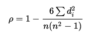
Where n is the number of measured pairs X and Y. The coefficient value can vary from -1 to 1. A positive value indicates a direct dependence of the researched values, negative one means a reverse dependence. A zero value indicates that there is no dependency.

As an example, let's zoom in on one of the methods of determining the ADX trend on the EURUSD currency pair. The others will be calculated similarly and their results will be added to a table for better clarity. In our case, the measurement of the average values of the trend time is n=7, with pre-selected number of bars for the test (100, 200, 300, 500, 1,000, 1,500, 2,000). The following table shows the results of measurement of the values, their ranging, the range difference and squared range for calculating the coefficient:

Rx	X	Y	Ry	D(Rx-Ry)	D2
1	100	75.78	1	0	0
2	200	77.72	2	0	0
3	300	79.04	3	0	0
4	500	79.77	5	-1	1
5	1,000	79.49	4	-1	1
6	1,500	81.32	6	0	0
7	2,000	81.44	7	0	0

By inserting these values into the formula, we obtain the coefficient ρ=1-(6*2)/(7*(49-1)=0.96.

Next, we check the obtained value in the table of the critical coefficient values shown in Fig. 8, for n=7, and conclude that within this test there is a strong, directly proportional dependence between the average value of the trend and the value of the selected testing sample in the bars.

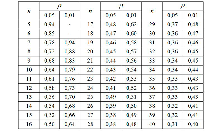
Fig.8 Critical values of the Spearman's rank correlation coefficient.

Next, we calculate the Spearman's coefficient for all trend identification methods for the selected EURUSD currency pair and display the results in a table.

Trend determination method	The Spearman coefficient value
ADX	0.96
ColorBBCount	0.89
Percentage of Trend	0.68
RSI Filter	-0.68
ZigZagTrendDetector	-0.07

What do the results say? The first three methods of determining the trend gave a direct dependence of the average trend value on the history depth, RSI Filter, on the contrary, demonstrated an inverse relationship, while the ZigZag indicator showed that the final result does not depend on the size of sample series. Let's calculate the coefficients for other instruments involved in the testing and also summarize the results in the table.

Trend determination method	EURUSD	USDCHF	USDJPY	GBPUSD	GOLD-6.17	#MCD
ADX	0.96	-0.61	-0.75	0.96	-0.86	0.93
ColorBBCount	0.89	0.46	-0.11	-0.14	-0.64	0.79
Percentage of Trend	0.68	0.93	0.11	0.29	0.89	1
RSI Filter	-0.68	1	0.04	0.79	-1	0.89
ZigZagTrendDetector	-0.07	0	0.96	0.96	0.36	0.32

Based on the obtained results, the following conclusions can be drawn for each of the trading instruments.

EURUSD. In three of the five trend analyzing methods, there is a strong correlation: The deeper the history, the larger will be its ratio of the trend state of the market.
USDCHF. Similar to the previous instrument: earlier, the share of the trend state of the market was higher than now.
USDJPY. Here, there is no relationship between the change in the sample size and the final value. The nature of the movement and dynamics of this market have not changed much.
GPBUSD. In four out of five methods, there is a directly proportional dependence between the ratio of the trend and the sample size. We also conclude that, on this pair, the share of the trend state of the market in the past was higher than today.
GOLD-6.17. We observed no dependence on the size of the sample.
#MCD. Dependence is present in all five cases (prominent - in four of these). This also indicates strong and long trends in the past. The closer the history to today, the less will be the duration and occurrence of strong movements on the chosen market.

To verify the reliability of the obtained results, let's consider the charts of the tested instruments on a large timeframe and for a long history period. This will give an idea of whether the nature of trend movements is changing. For the study, let's consider a weekly timeframe and try to identify the characteristic segments of trend and flat.

1. EURUSD

Consider the picture below. It shows the EURUSD currency pair from 1995 to the present.

Weekly EURUSD char, 1995-2017

Here, three zones denote the characteristic features of the market:

First zone shows a general long-term downward trend with slight pullbacks. Pay attention to the duration and strength of the trend.
Second zone is almost complete opposite of the first in terms of its movement, but the trend similar strength and duration is similar to the first one. As we can see, these two movements occurred between 1995 and mid-2007.
On the third and fourth marked zones, the strength and duration of trend movements is in heavy decline. On the historic scale, modern trends look more like sideway movements.

These observations suggest that the calculation of the Spearman's rank correlation coefficients for the selected methods of determining the trend reliably shows the current character of the changing trend/flat ratio.

2. USDJPY

The calculation of the correlation coefficients for this symbol showed neither dependence on the nature of the change nor correlation between the trend and the time. Fig. 10 clearly shows that since early 1995 there is a prominent, strong upward movement, followed by a protracted period of significantly shorter trends with much smaller amplitude. In the second part of the figure (with a descending trend followed by an ascending trend) there are noticeable frequent flat movements that last for several months.

Fig.10 The weekly chart USDJPY 1995-2017.

Therefore, in this case the Spearman's rank correlation coefficients also correctly describe the absence of dependency between the time period and the trend/flat ratio.

3. #MCD.

On stocks, the correlation was observed in all five methods of determining the trend. Fig. 11 shows that in the past, the stock moved up without significant pullbacks or protracted flat states. Also, we clearly see what movement and what ratio of trend/flat zones has been dominant in the recent past and to this day.

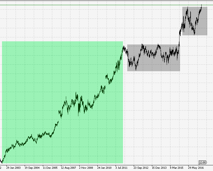
Fig.11 #MCD stock, 2003-2017.

Therefore, here, too, the calculation of the Spearman's rank correlation coefficients is completely justified and presents a picture characterizing a strong change in the trend/flat ratio towards the flat state. The general trend of the studied markets shows that the markets change both in terms of movement and in terms of the character of this movement. They become erratic, more dynamic and less predictable. This can be proved by the results obtained in this article: The trend/flat ratio has shifted towards the sideways movements; earlier the trend was more visible and obvious than it is today.

Conclusions

For a better presentation of tests, the total values of all the tested instruments are shown as a table.

Tested Symbol	Average value of the trend time, %
EURUSD	62.54
USDCHF	62.27
USDJPY	63.05
GBPUSD	60.68
GOLD-6.17	59.55
#MCD	59.71

Based on the summary table of test results, we can conclude the following: for given test conditions, the average market value in the trend state is about 60%, while on the time scale from the past to the present the trend/flat ratio shifts toward the flat, gradually approaching the initial assumption of the 30:70 ratio.

What do the results tell us?

The markets are more dynamic, the trend/flat phase fluctuation occurs increasingly often.
Long trend periods are changing into shorter fluctuations; the character of their movement is less clear than before.
Accordingly, market dynamics, movements and phases have become more complex.

Conclusion

The attached archive contains all the listed files, which are located in appropriate folders. For their proper operation, you only need to save the MQL5 folder into the terminal root folder.

Programs used in the article:

#	Name	Type	Description
1	TrendCount.mq5	Expert	Testing tool
2	TrendCountUI.mqh	Library	User interface class
3	ColorBBCandles.mq5	Indicator	Trend power and direction indicator (based on Bollinger Bands)
4	percentageoftrend.mq5	Indicator	Trend/flat state calculation indicator.
5	rsifilter.mq5	Indicator	RSI Indicator (histogram) with pre-set overbought/oversold levels.
6	ZigZagTrendDetector.mq5	Indicator	Indicator for determining the trend using the standard ZigZag.

Translated from Russian by MetaQuotes Ltd.
Original article: https://www.mql5.com/ru/articles/3188

Attached files |

Download ZIP

MQL5.zip (1693.17 KB)

Warning: All rights to these materials are reserved by MetaQuotes Ltd. Copying or reprinting of these materials in whole or in part is prohibited.