

Automatic Differentiation: Exact Gradients Without a Step Size
 69
 0

Contents
- Introduction
- The step size you should not have to choose
- Forward mode: a number that carries its own derivative
- Reverse mode: record the calculation, then walk it backwards
- A tape of parent slots and local partials
- Growing the tape without making the recording quadratic
- The sweep
- ADVar, the type that does the recording
- Checking that the derivatives are actually right
- Closed forms, and the two modes against each other
- Against jax, and the floor the comparison cannot get under
- What a gradient costs as the parameter count grows
- Putting it to work: an exact Jacobian for ALGLIB
- The model and the two callbacks
- Which mode fills a Jacobian faster
- The difference step that turned out not to matter
- What an exact Jacobian does not fix
- The same fit, running on a chart
- The edges AD does not smooth over
- Conclusion
Introduction
Plenty of useful work in a trading terminal comes down to minimizing something. You fit a decay model to an autocorrelation curve, calibrate a volatility surface, tune a small network's weights, or find the parameter set that best explains a spread. Every one of those is handed to an optimizer, and every serious optimizer wants a derivative.
There are three ways to give it one. You can derive the gradient by hand, which is exact and fast and goes wrong the moment the model changes. You can let the optimizer build one from finite differences, which is what most MQL5 code does and which quietly introduces a number you now have to choose: the step size. Or you can compute the derivative alongside the function itself, by arithmetic rather than approximation. That third option is automatic differentiation, the subject here.
The step size is worth dwelling on, because it is the part that hides. A difference quotient fails in two ways: a large step measures a chord, not a tangent. A small step loses significant digits when subtracting nearly equal doubles. The best step lies in between, depends on the function and the point and the scale of the variable, and nothing tells you when you have picked badly. The optimizer converges either way. It just converges somewhere slightly different.
Automatic differentiation eliminates the step-size choice. Both modes built here produce a derivative exact up to floating point rounding, with no approximation step and no parameter to tune. What follows includes the full library and the measurements behind each claim. It also shows three results that contradict common advice:
- Reverse mode, the usual advice for a gradient, is the wrong shape for a least-squares Jacobian.
- AD is slower than finite differences below about five parameters.
- An exact Jacobian does not fix a model that was never identifiable.
The library is six files and about three thousand lines. Its only dependency is ALGLIB, which ships with MetaTrader 5; the Python cross-check is optional.
The step size you should not have to choose
Before any of the code, here is what the code is for. The test script computes one gradient two ways: using central differences with ten step sizes spanning nine orders of magnitude, and using automatic differentiation. The function is a six-variable sum of products of exponentials, chosen because it has no special structure to flatter either method.
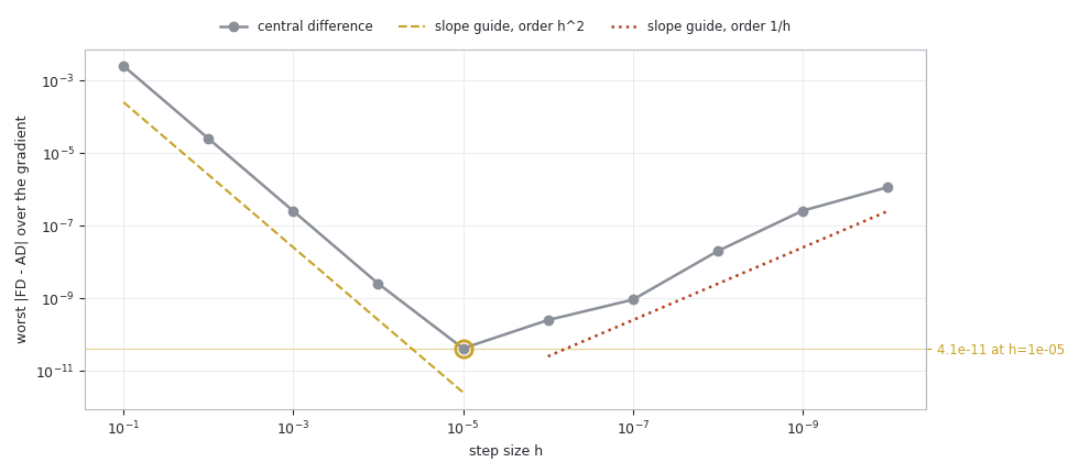
Fig. 1. The two errors a difference quotient trades off, measured on a six-variable gradient; the best step is a floor, not an exact answer
The left limb is truncation. At a step of 0.1 the quotient measures a chord across a curved function and lands 2.505e-03 away, and every factor of ten shrinks that by a hundred, the order h^2 behavior of a central difference. The right limb is cancellation. Below 1e-5 the two function values agree in so many leading digits that their difference is mostly rounding noise, and dividing that noise by a tiny h magnifies it. By 1e-10 the error is back up to 1.136e-06, worse than at h=1e-3.
The bottom of the V sits at h=1e-5, where the worst component is 4.113e-11 away from the AD answer. That is the best a central difference can do here, and it took ten sweeps to find it. In production you do not run that sweep. You pick a step and live with whatever limb you landed on.
Here is the section as the script prints it.
SECTION 3  the step size tradeoff that AD does not have
    h=1e-01   worst |FD - AD| = 2.505e-03
    h=1e-02   worst |FD - AD| = 2.503e-05
    h=1e-03   worst |FD - AD| = 2.503e-07
    h=1e-04   worst |FD - AD| = 2.504e-09
    h=1e-05   worst |FD - AD| = 4.113e-11
    h=1e-06   worst |FD - AD| = 2.475e-10
    h=1e-07   worst |FD - AD| = 9.033e-10
    h=1e-08   worst |FD - AD| = 1.977e-08
    h=1e-09   worst |FD - AD| = 2.555e-07
    h=1e-10   worst |FD - AD| = 1.136e-06
  best case central difference: h=1e-05 at 4.113e-11
  AD needed no h at all and carries no such curve
  [PASS] FD meets AD at its best h          got 4.1125103322769974e-11  want 0  rel 4.113e-11
The AD gradient in that comparison has no step size, no sweep, and no curve. Where a closed form exists to check it against, as in the next sections, it agrees to 2.878e-16 relative, one or two units in the last place of a double-precision number. That is what this article delivers. The rest explains how.
Forward mode: a number that carries its own derivative
The first mode rests on an idea that takes one line to state. Replace every real number in your calculation with a pair, a value and a derivative, and define arithmetic on pairs so the derivative half updates by the chain rule whenever the value half does. Nothing is approximated, nothing is symbolically manipulated. The derivative simply travels along.
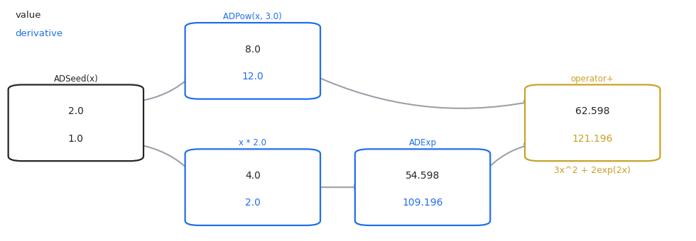
Fig. 2. Every box carries a value over a derivative; seeding the input derivative with 1.0 makes the output derivative the answer
Seeding the input with a derivative of 1.0 says "differentiate with respect to this one". By the time the calculation reaches the final sum, the derivative half holds 121.196, which is 3x^2 + 2exp(2x) at x=2. Nobody wrote that expression anywhere. It is what the arithmetic produced.
The dual number, and the rules that fall out of it
The formal version is a number written v + d*eps, where eps is a symbol with eps*eps = 0. Multiply two of them out and the eps squared term vanishes:
(a + a'eps)(b + b'eps) = ab + (ab' + a'b)eps
The coefficient of eps is the product rule. It was not coded; it is what survives once the squared term is dropped. The same happens for every operation, which is why the struct below is so short. Here are the two operators where it is easiest to see.
//+------------------------------------------------------------------+
//| Product rule, which nobody had to code: it is what remains once  |
//| the eps squared term is dropped                                  |
//+------------------------------------------------------------------+
ADDual ADDual::operator*(const ADDual &o) const
  {
   ADDual r;
   r.Set(v * o.v, v * o.d + d * o.v);
   return(r);
  }

//+------------------------------------------------------------------+
//| Quotient rule                                                    |
//+------------------------------------------------------------------+
ADDual ADDual::operator/(const ADDual &o) const
  {
   ADDual r;
   r.Set(v / o.v, (d * o.v - v * o.d) / (o.v * o.v));
   return(r);
  }
Multiplication returns v * o.v for the value and v * o.d + d * o.v for the derivative; division carries the quotient rule in the same shape. Both are exact rearrangements of the definition rather than approximations of it, which is why there is no h anywhere in this file.
The struct declares one method per operation, plus an overload of each taking a plain double so a constant needs no dual number wrapped around it.
//+------------------------------------------------------------------+
//| ADDual                                                           |
//|                                                                  |
//|  Forward mode. A number carried together with its derivative as  |
//|  v + d*eps, where eps*eps = 0. Every operator below drops the    |
//|  eps squared term, and what survives is the differentiation rule |
//|  itself: the product rule falls out of multiplication.           |
//+------------------------------------------------------------------+
struct ADDual
  {
   double            v;          // the value
   double            d;          // the derivative that rides along

   void              Set(const double value, const double deriv);
   ADDual            operator+(const ADDual &o)  const;
   ADDual            operator-(const ADDual &o)  const;
   ADDual            operator*(const ADDual &o)  const;
   ADDual            operator/(const ADDual &o)  const;
   ADDual            operator+(const double k)   const;
   ADDual            operator-(const double k)   const;
   ADDual            operator*(const double k)   const;
   ADDual            operator/(const double k)   const;
  };
Two free functions do the seeding. ADSeed sets the derivative to 1.0, marking the variable you are differentiating with respect to; ADFixed sets it to 0.0, marking everything else constant for this pass. A gradient in n variables therefore needs n passes, which is forward mode's defining cost.
The elementary functions
Beyond arithmetic, each elementary function needs its own rule, because the chain rule is applied by hand exactly once, where the function is defined. After that it composes for free.
//+------------------------------------------------------------------+
//| exp, whose derivative is itself                                  |
//+------------------------------------------------------------------+
ADDual ADExp(const ADDual &x)
  {
   ADDual r;
   double e = MathExp(x.v);
   r.Set(e, e * x.d);
   return(r);
  }

//+------------------------------------------------------------------+
//| Natural logarithm                                                |
//+------------------------------------------------------------------+
ADDual ADLog(const ADDual &x)
  {
   ADDual r;
   r.Set(MathLog(x.v), x.d / x.v);
   return(r);
  }

//+------------------------------------------------------------------+
//| Square root, whose slope blows up at zero and is left to do so   |
//+------------------------------------------------------------------+
ADDual ADSqrt(const ADDual &x)
  {
   ADDual r;
   double s = MathSqrt(x.v);
   r.Set(s, x.d / (2.0 * s));
   return(r);
  }
ADExp is the neatest case: the derivative of exp is exp, so the value just computed is also the local factor and one call to MathExp serves both halves. ADSqrt does nothing to protect against a zero argument, which is deliberate; the slope of the square root really is infinite there, and hiding that would be worse than reporting it.
The full set is small enough to list. Each exists in two forms, one taking an ADDual, one an ADVar, with the same name and meaning.
| Function | Local derivative recorded | Note |
|---|---|---|
| ADExp | exp(x) | reuses its own value |
| ADLog | 1 / x | undefined at and below zero |
| ADSqrt | 1 / (2 sqrt(x)) | slope diverges at zero |
| ADSin | cos(x) | evaluates cos as well |
| ADCos | -sin(x) | evaluates sin as well |
| ADPow | n * x^(n-1) | constant exponent only |
| ADTanh | 1 - tanh(x)^2 | reuses its own value |
| ADAbs | sign(x) | zero at zero, by convention |
That is the whole of forward mode. It is roughly two hundred lines, it has no state, and it costs one pass per input variable.
Reverse mode: record the calculation, then walk it backwards
Forward mode's cost is proportional to the number of inputs, fine for one or two and painful for a hundred. Reverse mode inverts that: it evaluates the function once, recording what it did, then propagates a derivative backwards from the output to every input in one pass whose cost does not depend on how many inputs there are.
The recording is called a tape, and the design decision that makes this library short is what goes on it. The tape stores no opcodes. Each node stores only its parent slots and the local partials, computed during the forward pass while operand values are available. The backward sweep therefore never asks what operation produced a node. It multiplies and adds.
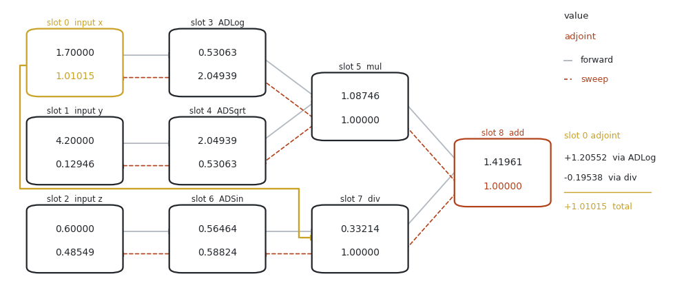
Fig. 3. Slot 0 is reached by two routes, so its adjoint is a sum; that accumulation is the only thing the sweep has to get right
A tape of parent slots and local partials
The class is five per-slot arrays, a separate array of input slots, and four counters. There is no node struct, because flat arrays of doubles and ints are friendlier to the cache than an array of small objects, and the tape is the hot data structure in any fitting loop.
//+------------------------------------------------------------------+
//| CADTape                                                          |
//|                                                                  |
//|  Reverse mode. The forward pass records one node per operation,  |
//|  storing only the parent slots and the local partials, which are |
//|  free to compute while the values are in hand. The reverse sweep |
//|  then needs no operation codes and no second evaluation.         |
//+------------------------------------------------------------------+
class CADTape
  {
private:
   int               m_a[];       // first parent, -1 when there is none
   int               m_b[];       // second parent, -1 for unary nodes
   double            m_pa[];      // d(this)/d(first parent)
   double            m_pb[];      // d(this)/d(second parent)
   double            m_adj[];     // adjoint scratch, reused across sweeps
   int               m_input[];   // slots that were declared as inputs
   int               m_count;     // nodes recorded
   int               m_capacity;  // nodes allocated
   int               m_inputs;    // inputs declared
   int               m_inputCap;  // input slots allocated

   void              Reserve(const int needed);
   void              ReserveInputs(const int needed);

public:
                     CADTape(void);
   void              Reset(void);
   int               PushInput(void);
   int               PushUnary(const int a, const double pa);
   int               PushBinary(const int a, const int b,
                                const double pa, const double pb);
   bool              Gradient(const int outSlot, double &grad[]);
   int               Count(void)      const { return(m_count);  }
   int               InputCount(void) const { return(m_inputs); }
  };
The arrays hold, per slot, two parents, the two local partials, and a scratch adjoint reused between sweeps. A parent index of -1 means none, which marks leaves and unary nodes. m_input lists the slots declared as inputs, so the gradient comes back in declaration order rather than tape order.
For the function in Fig. 3 at x=1.7, y=4.2 and z=0.6, the recording comes out as nine slots. Reading the table across is reading the five arrays down.
| Slot | What produced it | m_a | m_b | m_pa | m_pb |
|---|---|---|---|---|---|
| 0 | ADInput(x) | -1 | -1 | 0 | 0 |
| 1 | ADInput(y) | -1 | -1 | 0 | 0 |
| 2 | ADInput(z) | -1 | -1 | 0 | 0 |
| 3 | ADLog(x) | 0 | -1 | 0.58824 | 0 |
| 4 | ADSqrt(y) | 1 | -1 | 0.24398 | 0 |
| 5 | slot 3 * slot 4 | 3 | 4 | 2.04939 | 0.53063 |
| 6 | ADSin(z) | 2 | -1 | 0.82534 | 0 |
| 7 | slot 6 / slot 0 | 6 | 0 | 0.58824 | -0.19538 |
| 8 | slot 5 + slot 7 | 5 | 7 | 1 | 1 |
Slot 0 appears as a parent twice, at slot 3 and at slot 7, because x is used in two places. That is the case a gradient implementation has to handle, and the sweep handles it by accumulating rather than assigning: x gets 1.20552 through the logarithm and -0.19538 through the division, and the answer is their sum, 1.01015.
Growing the tape without making the recording quadratic
A tape gains one node per operation, so it is appended to constantly. Calling ArrayResize with the exact new size each time would reallocate and copy on every append, making a function with N operations cost O(N^2) to record. Capacity doubling makes an append amortized constant.
//+------------------------------------------------------------------+
//| Capacity doubling. A tape grows once per operation, so resizing  |
//| by one here would make every recorded function quadratic         |
//+------------------------------------------------------------------+
void CADTape::Reserve(const int needed)
  {
   if(needed <= m_capacity)
      return;
   int cap = (m_capacity == 0 ? 256 : m_capacity);
   while(cap < needed)
      cap *= 2;
   ArrayResize(m_a,   cap);
   ArrayResize(m_b,   cap);
   ArrayResize(m_pa,  cap);
   ArrayResize(m_pb,  cap);
   ArrayResize(m_adj, cap);
   m_capacity = cap;
  }
The three push methods are the only way nodes get onto the tape, and each returns the slot it wrote so the caller can refer to it later.
//+------------------------------------------------------------------+
//| A leaf the gradient will be reported for                         |
//+------------------------------------------------------------------+
int CADTape::PushInput(void)
  {
   Reserve(m_count + 1);
   ReserveInputs(m_inputs + 1);
   m_a[m_count] = -1;
   m_b[m_count] = -1;
   m_pa[m_count] = 0.0;
   m_pb[m_count] = 0.0;
   m_input[m_inputs] = m_count;
   m_inputs++;
   m_count++;
   return(m_count - 1);
  }

//+------------------------------------------------------------------+
//| One operation with one parent, such as exp or a scalar multiply  |
//+------------------------------------------------------------------+
int CADTape::PushUnary(const int a, const double pa)
  {
   Reserve(m_count + 1);
   m_a[m_count] = a;
   m_b[m_count] = -1;
   m_pa[m_count] = pa;
   m_pb[m_count] = 0.0;
   m_count++;
   return(m_count - 1);
  }

//+------------------------------------------------------------------+
//| One operation with two parents, such as a product                |
//+------------------------------------------------------------------+
int CADTape::PushBinary(const int a, const int b,
                        const double pa, const double pb)
  {
   Reserve(m_count + 1);
   m_a[m_count] = a;
   m_b[m_count] = b;
   m_pa[m_count] = pa;
   m_pb[m_count] = pb;
   m_count++;
   return(m_count - 1);
  }
Reset sets the two counters to zero and touches nothing else, so the arrays keep the memory they have claimed. A fitting loop that records the same function ten thousand times pays for allocation once and never again.
The sweep
Everything above exists to make this function short. Seed the output slot with an adjoint of 1.0, walk the tape backwards, and hand each node's adjoint down to its parents scaled by the stored partials.
//+------------------------------------------------------------------+
//| The reverse sweep. Seed the output with one, walk the tape       |
//| backwards, and every input holds its own derivative at the end.  |
//| False means the slot is not on this tape and grad is untouched.  |
//| One pass, whatever the number of inputs.                         |
//+------------------------------------------------------------------+
bool CADTape::Gradient(const int outSlot, double &grad[])
  {
   if(outSlot < 0 || outSlot >= m_count)
      return(false);
   ArrayFill(m_adj, 0, m_count, 0.0);
   m_adj[outSlot] = 1.0;
//--- backwards, so every node is reached only after everything that
//--- consumes it has already handed down its share
   for(int i = m_count - 1; i >= 0; i--)
     {
      double g = m_adj[i];
      //--- skipping a zero adjoint is not only cheaper, it keeps a node
      //--- with an infinite partial from turning the sweep into NaN
      if(g == 0.0)
         continue;
      int a = m_a[i];
      if(a >= 0)
         m_adj[a] += g * m_pa[i];
      int b = m_b[i];
      if(b >= 0)
         m_adj[b] += g * m_pb[i];
     }
//--- resized in both directions, so ArraySize(grad) is always the input
//--- count and a reused array can never carry a stale tail
   ArrayResize(grad, m_inputs);
   for(int k = 0; k < m_inputs; k++)
      grad[k] = m_adj[m_input[k]];
   return(true);
  }
Walking backwards is what makes a single pass sufficient. A node can only have been built from slots with smaller indices, so by the time the loop reaches slot i, every node that consumes it has already added its share. The adjoint is complete when it is read.
The zero adjoint skip is not only an optimization. A node whose subtree does not reach the output has an adjoint of exactly zero, and if it also carries an infinite partial, which ADSqrt at zero would, the product is a NaN that spreads through the sweep. Skipping the multiply keeps a value nobody asked about from poisoning the values somebody did.
The output array is resized unconditionally. After a successful call, ArraySize(grad) equals the declared input count, and a reused array cannot retain stale elements.
ADVar, the type that does the recording
The tape cannot record anything by itself. That is the job of a second number type, which looks like the dual number but carries a slot index instead of a derivative.
//+------------------------------------------------------------------+
//| ADVar                                                            |
//|                                                                  |
//|  Reverse mode variable: a value plus the slot it occupies on the |
//|  tape. The value travels with it so each operator can work out   |
//|  its own partials on the spot, which is why the reverse sweep    |
//|  never has to know which operation produced a node.              |
//+------------------------------------------------------------------+
struct ADVar
  {
   double            v;          // the value, as in an ordinary forward pass
   int               slot;       // where this value sits on the tape

   void              Set(const double value, const int tapeSlot);
   ADVar             operator+(const ADVar &o)   const;
   ADVar             operator-(const ADVar &o)   const;
   ADVar             operator*(const ADVar &o)   const;
   ADVar             operator/(const ADVar &o)   const;
   ADVar             operator+(const double k)   const;
   ADVar             operator-(const double k)   const;
   ADVar             operator*(const double k)   const;
   ADVar             operator/(const double k)   const;
  };
The value travels with the variable for one reason: each operator needs the operand values to work out its own local partials, at the moment the operation happens. Look at multiplication and division.
//+------------------------------------------------------------------+
//| A product hands each parent the other one's value                |
//+------------------------------------------------------------------+
ADVar ADVar::operator*(const ADVar &o) const
  {
   ADVar r;
   r.Set(v * o.v, g_ADTape.PushBinary(slot, o.slot, o.v, v));
   return(r);
  }

//+------------------------------------------------------------------+
//| A quotient stores both partials directly, so the reverse sweep   |
//| never has to re-form the quotient rule                           |
//+------------------------------------------------------------------+
ADVar ADVar::operator/(const ADVar &o) const
  {
   ADVar r;
   r.Set(v / o.v, g_ADTape.PushBinary(slot, o.slot,
                                      1.0 / o.v, -v / (o.v * o.v)));
   return(r);
  }
The product pushes a binary node whose partials are the two operand values, swapped, because d(ab)/da is b. The quotient pushes 1/b and -a/b^2. Both are computed on the spot and stored as plain doubles, and the sweep reading them back has no idea which line produced them.
One helper exists purely because of a language constraint. MQL5 overloads operators as struct methods, so the left operand has to be the struct type. Writing 1.0 - x where x is an ADVar has no overload to bind to, and a free operator- taking a double on the left is rejected. The Rosenbrock function needs exactly that expression, so a constant gets its own slot.
//+------------------------------------------------------------------+
ADVar ADConst(const double value)
  {
   ADVar r;
   r.Set(value, g_ADTape.PushUnary(-1, 0.0));
   return(r);
  }
It is a node with no parent and a partial of zero. It costs one tape slot and it makes the constant a first class operand.
Checking that the derivatives are actually right
A gradient implementation that is subtly wrong is worse than none, because the optimizer usually still converges, just somewhere slightly different, and nothing complains. So the library is checked three ways: against derivatives known on paper, against itself with the two modes compared, and against an established implementation in another language.
Closed forms, and the two modes against each other
The first two sections differentiate functions whose derivatives can be written down, so the tolerance can sit near machine epsilon rather than being chosen to make a test pass. It is 1e-14 relative.
SECTION 1  analytic ground truth (forward and reverse)
  [PASS] fwd  x^3+exp(2x)                   got 121.19630006628847  want 121.19630006628847  rel 0.000e+00
  [PASS] rev  x^3+exp(2x)                   got 121.19630006628847  want 121.19630006628847  rel 0.000e+00
  [PASS] fwd  log(x)sqrt(x)                 got 0.97045163417636893  want 0.97045163417636904  rel 1.144e-16
  [PASS] rev  log(x)sqrt(x)                 got 0.97045163417636893  want 0.97045163417636904  rel 1.144e-16
  [PASS] fwd  sin(x)/x                      got -0.19289195680341226  want -0.19289195680341226  rel 0.000e+00
  [PASS] rev  sin(x)/x                      got -0.1928919568034122  want -0.19289195680341226  rel 2.878e-16
  [PASS] fwd  tanh(3x)                      got 0.91505998862222648  want 0.91505998862222648  rel 0.000e+00
  [PASS] rev  tanh(3x)                      got 0.91505998862222648  want 0.91505998862222648  rel 0.000e+00
SECTION 2  multi parameter gradients
  [PASS] rev  Rosenbrock d/dx               got -215.59999999999997  want -215.59999999999999  rel 1.318e-16
  [PASS] rev  Rosenbrock d/dy               got -87.999999999999986  want -87.999999999999986  rel 0.000e+00
  [PASS] fwd  Rosenbrock d/dx               got -215.59999999999997  want -215.59999999999999  rel 1.318e-16
  [PASS] fwd  Rosenbrock d/dy               got -87.999999999999986  want -87.999999999999986  rel 0.000e+00
  [PASS] rev  log*sqrt+sin/x d/dx           got 1.0101456010488681  want 1.0101456010488681  rel 0.000e+00
  [PASS] rev  log*sqrt+sin/x d/dy           got 0.12946003723003116  want 0.12946003723003116  rel 0.000e+00
  [PASS] rev  log*sqrt+sin/x d/dz           got 0.48549153818216373  want 0.48549153818216373  rel 0.000e+00
Every one lands at or below 2.878e-16, one or two units in the last place of a double-precision number. The Rosenbrock case matters more than its size suggests: it is the first function with two inputs, so forward mode's one sweep per variable and reverse mode's one sweep total are both exercised and required to agree.
The last group is the accumulation case from Fig. 3, where x is reached by two routes. If the sweep assigned adjoints instead of adding them, d/dx would come out as 1.20552 or -0.19538 instead of 1.01015. The test would fail loudly. It does not.
Against jax, and the floor the comparison cannot get under
Agreeing with your own arithmetic is not independent evidence. The export script evaluates seven functions in both modes and writes the inputs next to the gradients at %.17g, so every double round trips exactly; a Python script differentiates the same seven with jax and compares.
Two things about that comparison are easy to get wrong. First, jax defaults to single precision. On x^3 + exp(2x) at x=2 that alone puts the reference gradient 4.255e-06 away from the true value, swamping every difference the script is trying to measure. Enabling 64-bit mode is mandatory.
Second, the tolerance cannot be zero. MQL5's MathExp and XLA's jnp.exp are different implementations of the same function and are entitled to disagree in the last bit. On exp(-1.05), MQL5 and Python's math.exp return the identical double; jnp returns the one next door.
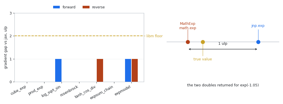
Fig. 4. The two libraries differ by one unit in the last place on exp(-1.05), and the true value lies between them, so a nonzero floor is a property of the comparison rather than of the tape
Checked against a 60-digit reference, the platform library returns the correctly rounded double here and jnp is the one that is off. The same holds at tanh(-0.105), where the gap is two units. So the script measures that floor itself, over ten arguments and three functions, and prints it beside the results rather than assuming a value.
jax 0.11.1, x64=True
14 rows from ad_gradients.csv
transcendental floor: platform libm vs XLA differ by up to 2 ulp (worst at tanh(-0.105))
gradients are therefore allowed 2 ulp

  [PASS] cube_exp       forward  n=1  value 0 ulp  grad 0 ulp (limit 2)
  [PASS] cube_exp       reverse  n=1  value 0 ulp  grad 0 ulp (limit 2)
  [PASS] prod_exp       forward  n=2  value 0 ulp  grad 0 ulp (limit 2)
  [PASS] prod_exp       reverse  n=2  value 0 ulp  grad 0 ulp (limit 2)
  [PASS] log_sqrt_sin   forward  n=3  value 0 ulp  grad 1 ulp (limit 2)
  [PASS] log_sqrt_sin   reverse  n=3  value 0 ulp  grad 0 ulp (limit 2)
  [PASS] rosenbrock     forward  n=2  value 0 ulp  grad 0 ulp (limit 2)
  [PASS] rosenbrock     reverse  n=2  value 0 ulp  grad 0 ulp (limit 2)
  [PASS] tanh_cos_div   forward  n=2  value 0 ulp  grad 0 ulp (limit 2)
  [PASS] tanh_cos_div   reverse  n=2  value 0 ulp  grad 1 ulp (limit 2)
  [PASS] expsum_chain   forward  n=6  value 0 ulp  grad 0 ulp (limit 2)
  [PASS] expsum_chain   reverse  n=6  value 0 ulp  grad 0 ulp (limit 2)
  [PASS] expmodel       forward  n=5  value 2 ulp  grad 1 ulp (limit 2)
  [PASS] expmodel       reverse  n=5  value 2 ulp  grad 1 ulp (limit 2)

  worst reverse-mode disagreement : 1 ulp
  worst forward-mode disagreement : 1 ulp
  transcendental floor            : 2 ulp
  the AD gap is at or below the floor, so nothing here is
  attributable to the tape
  14 passed, 0 failed
The worst disagreement in either mode is one unit in the last place, against a measured floor of two. The gradients are as close to jax as two implementations of exp are to each other, which is as close as this comparison can get. Reporting it in ulp rather than as a relative error is what makes that checkable.
What a gradient costs as the parameter count grows
The headline claim for reverse mode is that one sweep returns the whole gradient, so its cost tracks a single function evaluation however many parameters there are, while differences need one evaluation per parameter at least. The test script measures that: each timing grows a batch until it exceeds 2000 microseconds, reports the fastest of seven, and prints the batch sizes so the numbers can be audited rather than trusted.
Every nanosecond and millisecond figure in this article came off one machine, so read the absolute times as that machine's rather than as the method's: an Intel Core i5-8265U at 1.60 GHz, four cores and eight threads with AVX2, under Windows 11 build 26200. The code was compiled by MetaEditor for its X64 Regular target and run as a script on a EURUSDm H1 chart rather than in the Strategy Tester, on MetaTrader 5 build 6182 for the test script and build 6140 for the fitting script. The counted quantities, batch sizes and residual evaluations, are exact and reproduce run to run. The clock readings do not: they are one measurement each and move by tens of percent between runs, which is why the comparisons below are argued from a gap rather than from a digit.
SECTION 4  cost against parameter count
  timing: min of 7 batches, batch sized to exceed 2000 us
     n   nodes     f() ns     AD ns      FD ns   FD/AD   AD/f()   batches f/AD/FD
     2       7       53.2     536.9      273.3     0.5    10.10   65536/4096/8192
     5      19      110.5     806.2      837.9     1.0     7.30   16384/4096/2048
    10      39      218.9    2070.3     2785.2     1.3     9.46   8192/1024/512
    20      79      241.1    3603.5    13882.8     3.9    14.95   8192/512/256
    50     199     1179.7    4980.5    67375.0    13.5     4.22   2048/256/32
   100     399     1202.6    9625.0   243875.0    25.3     8.00   2048/256/8
  nodes grow linearly in n, which is the tape's memory cost
  AD/f() went from 10.10 at n=2 to 8.00 at n=100
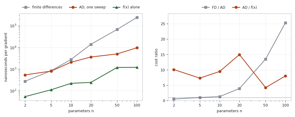
Fig. 5. The cost of automatic differentiation relative to one function call does not grow with the parameter count, while the cost of finite differences does
The right panel carries the two claims worth arguing about. AD / f(x) is the interesting one: it wanders between 4.2 and 15.0 across the sweep with no direction in n, and that absence of a trend is the property being asserted. Where it lands is wall clock noise on a working machine and moves between runs, so only the order of magnitude is worth reading. That order is not the textbook figure: the literature quotes three to four for reverse mode, and this library costs closer to ten because MQL5 operator overloading and a tape push each cost real time per operation, where the textbook counts arithmetic only.
FD/AD is the honest half. At n=2 it is 0.5: finite differences are twice as fast as AD, not slower. Break even arrives around n=5, where the ratio is 1.0. The advantage becomes large past n=20, at 13.5 times by n=50 and 25.3 by n=100. Below about five parameters AD is the wrong tool on cost grounds, and the argument for it there has to be exactness rather than speed.
The node count is the memory story: 7 nodes at n=2 and 399 at n=100, linear in n, each four numbers wide. A tape is not free, and for a function evaluated inside a tight loop over thousands of bars, that allocation is the thing to watch.
Putting it to work: an exact Jacobian for ALGLIB
A gradient library that only proves things about itself is not much use. ALGLIB ships with MetaTrader 5, and its Levenberg-Marquardt solver has two entry points: MinLMCreateV, which builds a Jacobian from finite differences using a step you supply, and MinLMCreateVJ, which asks you for the Jacobian. The second is normally where a reader gives up and derives by hand. This is what happens when AD supplies it.
The model and the two callbacks
The model is a constant plus K decaying exponentials, with 2K+1 parameters. Sums of exponentials are a classic ill-conditioned fit, which is why the quality of the Jacobian shows up in the result rather than being washed out.
y(t) = c + sum over k of a_k * exp(-b_k * t)ALGLIB asks for residuals through one callback and the Jacobian through another. The Jacobian callback is where both modes appear side by side, since the same matrix can be filled either way and the script switches at run time.
//+------------------------------------------------------------------+
//| Forward mode fills a Jacobian COLUMN per sweep and reverse mode  |
//| fills a ROW, so forward needs fewer sweeps when there is more    |
//| data than parameters. Both are exact; only the cost differs.     |
//+------------------------------------------------------------------+
void CFitJac::Jac(CRowDouble &x, CRowDouble &fi,
                  CMatrixDouble &jac, CObject &obj)
  {
   g_cbJac++;
   double p[];
   ArrayResize(p, g_n);
   for(int j = 0; j < g_n; j++)
      p[j] = x[j];

//--- forward mode: one sweep per parameter, each filling a column
   if(g_jacMode == JAC_FORWARD)
     {
      ADDual dp[];
      ArrayResize(dp, g_n);
      for(int j = 0; j < g_n; j++)
        {
         //--- seed parameter j and hold the rest fixed, so every derivative
         //--- coming back down this sweep is the one with respect to it
         for(int q = 0; q < g_n; q++)
            dp[q] = (q == j ? ADSeed(p[q]) : ADFixed(p[q]));
         for(int i = 0; i < g_m; i++)
           {
            ADDual s = dp[0];
            for(int k = 0; k < g_K; k++)
               s = s + dp[1 + k] * ADExp(dp[1 + g_K + k] * (-g_t[i]));
            jac.Set(i, j, s.d);
            if(j == 0)
               fi.Set(i, s.v - g_y[i]);
            g_resEval++;
           }
        }
      return;
     }

//--- reverse mode: one tape and one sweep for each residual
   for(int i = 0; i < g_m; i++)
     {
      g_ADTape.Reset();
      ADVar vp[];
      ArrayResize(vp, g_n);
      for(int q = 0; q < g_n; q++)
         vp[q] = ADInput(p[q]);
      ADVar s = vp[0];
      for(int k = 0; k < g_K; k++)
         s = s + vp[1 + k] * ADExp(vp[1 + g_K + k] * (-g_t[i]));
      double grad[];
      g_ADTape.Gradient(s.slot, grad);
      fi.Set(i, s.v - g_y[i]);
      for(int j = 0; j < g_n; j++)
         jac.Set(i, j, grad[j]);
      g_resEval++;
     }
  }
The forward branch loops over parameters outside and residuals inside, seeding one parameter at a time so each pass fills one column; the residual vector is filled only on the first pass, since it does not depend on which parameter is seeded. The reverse branch loops over residuals, resetting the tape, recording one residual, sweeping it and writing one full row.
Before any solver runs, the script checks the Jacobian on its own. That catches the failure mode where a callback is never invoked and the matrix stays full of zeros, which would look like a converged fit.
SECTION 0  the Jacobian itself, before any fitting
  largest |J| entry from forward mode: 1
  [PASS] forward Jacobian is not all zeros      err 0.000e+00
  worst forward vs reverse Jacobian entry: 2.124e-16
  [PASS] forward and reverse agree              err 2.124e-16
  worst |central difference - AD| over all m*n = 600: 4.767e-11
  [PASS] AD Jacobian matches differences        err 4.767e-11
  ALGLIB numerical (1e-6)    iters   35  nfunc  168  njac    9  SSE 1.020474e-02  resEval   20160     8.9 ms  term 2
  AD forward Jacobian        iters   15  nfunc   49  njac   16  SSE 1.020474e-02  resEval   13560     2.0 ms  term 2
  numerical: c=0.154 a=[0.9795 0.5052] b=[0.3037 0.03104]
  AD       : c=0.154 a=[0.9795 0.5052] b=[0.3037 0.03104]
  SSE 1.020474e-02 against a noise floor of m*sd^2 = 1.200000e-02  ratio 0.850
  [PASS] AD fit reaches the noise floor         err 1.496e-01
  worst |AD fit - truth| = 0.02047   window 119.0 covers 5.2 half lives of the slowest decay
  [PASS] AD fit recovers the truth              err 0.000e+00
  worst |AD - numerical| across parameters = 1.401e-10
  [PASS] both paths reach the same optimum      err 0.000e+00
Forward and reverse agree to 2.124e-16 over all 600 entries, and both agree with central differences to 4.767e-11, about where a difference quotient tops out. The two AD modes agree far more tightly with each other than either does with differences, the expected ordering and a sign that the differences are the loose end.
Which mode fills a Jacobian faster
This is the result that contradicts the pitch. The usual advice is that reverse mode is what you want for gradients, and it is, for a scalar objective. A Jacobian is not one. It is an m by n matrix, and the two modes fill it in different directions.
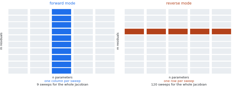
Fig. 6. A least-squares problem has far more residuals than parameters, which is the wrong shape for reverse mode
Least squares means many more residuals than parameters. With 120 data points and 9 parameters, forward mode needs 9 sweeps to fill the matrix and reverse mode 120. Reverse mode wins when outputs are few and inputs many, and a Jacobian inverts that condition.
SECTION 2  cost as the model grows
  --- K=1, n=3 parameters, m=120 points ---
  ALGLIB numerical (1e-6)    iters   12  nfunc   73  njac    6  SSE 1.032101e-02  resEval    8760     2.9 ms  term 2
  AD forward Jacobian        iters    7  nfunc   26  njac    8  SSE 1.032101e-02  resEval    5040     0.9 ms  term 2
  AD reverse Jacobian        iters    7  nfunc   26  njac    8  SSE 1.032101e-02  resEval    3120     1.4 ms  term 2
  --- K=2, n=5 parameters, m=120 points ---
  ALGLIB numerical (1e-6)    iters   16  nfunc   88  njac    5  SSE 1.030161e-02  resEval   10560     4.6 ms  term 2
  AD forward Jacobian        iters   18  nfunc   53  njac   19  SSE 1.030161e-02  resEval   15480     2.7 ms  term 2
  AD reverse Jacobian        iters   14  nfunc   40  njac   15  SSE 1.030161e-02  resEval    4800     1.8 ms  term 2
  --- K=3, n=7 parameters, m=120 points ---
  ALGLIB numerical (1e-6)    iters   72  nfunc  347  njac   15  SSE 1.028453e-02  resEval   41640    16.9 ms  term 2
  AD forward Jacobian        iters   29  nfunc   79  njac   30  SSE 1.028453e-02  resEval   31080     5.0 ms  term 2
  AD reverse Jacobian        iters   32  nfunc   90  njac   33  SSE 1.028453e-02  resEval   10800     7.9 ms  term 2
  --- K=4, n=9 parameters, m=120 points ---
  ALGLIB numerical (1e-6)    iters  705  nfunc 2787  njac   89  SSE 1.023642e-02  resEval  334440   160.1 ms  term 2
  AD forward Jacobian        iters  140  nfunc  351  njac  141  SSE 1.023642e-02  resEval  177480    20.6 ms  term 2
  AD reverse Jacobian        iters  141  nfunc  354  njac  142  SSE 1.023642e-02  resEval   42480    23.6 ms  term 2
  forward mode costs n sweeps per Jacobian, reverse mode m,
  so forward does fewer sweeps when there is more data than parameters
  resEval counts a forward and a reverse unit alike, though a reverse unit is a tape and a sweep
  the two ALGLIB entry points also run different internal modes, so iteration counts are not directly comparable
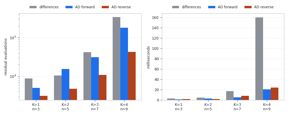
Fig. 7. Reverse mode does a quarter of the residual evaluations at K=4 and still takes slightly longer on the clock
The left panel is exact accounting: the script counts every residual evaluation, so those bars are deterministic and reproduce run to run. At K=4 the numerical path does 334,440, forward mode 177,480 and reverse mode 42,480. On count alone, reverse mode looks like the clear winner.
The right panel is wall clock, and it disagrees. Reverse mode takes 23.6 ms against forward mode's 20.6 ms, despite doing a quarter of the work by the other measure. A reverse sweep is not one residual evaluation: each of the 120 residuals costs a tape reset, a set of pushes and a backward pass, and that overhead exceeds the dual number arithmetic forward mode does instead. Both are far ahead of finite differences at 160.1 ms.
Three different measures are in play here and they do not agree, so they are worth keeping apart. The first is sweep count, and it is structural: forward mode needs n sweeps per Jacobian and reverse mode m, so forward does fewer of them when there are more residuals than parameters, which is every least-squares problem. The second is the resEval column, and it is not the same measure. It increments once per residual in both modes, so one forward unit is dual number arithmetic while one reverse unit is a tape reset, a recording pass and a backward sweep. Reverse mode counts lower at every K because of that definition rather than because it does less work. The third is wall clock, and it is the only one of the three that prices a reverse sweep at what it actually costs: forward mode leads at K=1, K=3 and K=4 and trails at K=2, where reverse finishes in 1.8 ms against 2.7 ms. One clock reading also moves by tens of percent between runs, so the gaps matter more than the digits.
The two modes did not take the same number of solver steps, so a raw total mixes what a Jacobian costs with how many of them ALGLIB asked for. The njac column divides that out. Per Jacobian call the readings are 0.113 ms against 0.175 at K=1, 0.142 against 0.120 at K=2, 0.167 against 0.239 at K=3 and 0.146 against 0.166 at K=4, forward mode first. They still carry the residual-only evaluations the solver interleaves, so they price a Jacobian call rather than the matrix fill alone. Dividing the iteration counts out does not remove the K=2 exception. It keeps it.
What that supports is narrower than the usual slogan. Over the sizes measured here, n=3 to n=9 against m=120, with this model and this implementation, forward mode is the one to reach for on a least-squares Jacobian, and K=2 is a standing exception rather than noise. What the numbers do not support is a rule covering every problem of that shape.
The difference step that turned out not to matter
Given Fig. 1, the obvious next claim is that a badly chosen difference step degrades the fit and AD rescues it. The script sweeps ALGLIB's diffstep over ten orders of magnitude to demonstrate that. It measures the opposite.
SECTION 3  sweeping the difference step ALGLIB is given
  AD forward Jacobian        iters   15  nfunc   49  njac   16  SSE 1.020474e-02  resEval   13560     1.7 ms  term 2
  numerical diffstep 1e-02   iters   43  nfunc  196  njac   10  SSE 1.020474e-02  resEval   23520     5.6 ms  term 2
  numerical diffstep 1e-04   iters   34  nfunc  151  njac    8  SSE 1.020474e-02  resEval   18120     4.5 ms  term 2
  numerical diffstep 1e-06   iters   35  nfunc  168  njac    9  SSE 1.020474e-02  resEval   20160     8.3 ms  term 2
  numerical diffstep 1e-08   iters   34  nfunc  155  njac    8  SSE 1.020474e-02  resEval   18600     4.1 ms  term 2
  numerical diffstep 1e-10   iters   35  nfunc  183  njac   10  SSE 1.020474e-02  resEval   21960     4.9 ms  term 2
  numerical diffstep 1e-12   iters   66  nfunc  260  njac   13  SSE 1.020474e-02  resEval   31200     8.6 ms  term 2
  AD reached SSE 1.020474e-02 with no step size to choose
  worst relative SSE gap across ten orders of diffstep: 3.901e-08
  MEASURED: the step size barely moves the answer here, because
  ALGLIB scales diffstep by each variable's own magnitude. The
  case for AD on this problem is cost and not having a knob,
  not rescuing a fit that differences would have got wrong.
  [PASS] numerical path is insensitive to diffstep err 0.000e+00
Across steps from 1e-2 down to 1e-12, the worst relative change in the final sum of squares is 3.901e-08. The fit is essentially unaffected, because ALGLIB scales the step by each variable's own magnitude, so a step that would be absurd for one parameter is silently made reasonable. What does change is the work: 18,120 residual evaluations at the best step, 31,200 at the worst.
So the case for AD here is cost and not having a knob, not rescuing an answer differences would have got wrong. The script reports that negative result rather than burying it, because a reader who adopts AD expecting better fits and gets identical ones deserves to have been told.
What an exact Jacobian does not fix
Everything so far was measured on synthetic data with a known answer. Real data carries the more useful lesson. Volatility clustering means the autocorrelation of absolute returns decays slowly, and how slowly is a fit away. The script builds that curve from H1 closes and fits it with one exponential, then two.
//+------------------------------------------------------------------+
//| Autocorrelation of absolute returns, the decay this fit targets  |
//+------------------------------------------------------------------+
bool BuildACF(const string sym, const int bars, const int lags)
  {
   double close[];
   int got = CopyClose(sym, PERIOD_H1, 0, bars, close);
//--- twenty pairs per lag, so even the longest lag is averaged over
//--- enough of them for its point on the curve to mean something
   if(got < lags * 20)
     {
      PrintFormat("  only %d bars of %s available, need %d - section skipped",
                  got, sym, lags * 20);
      return(false);
     }
//--- absolute log returns: the size of a move without its direction,
//--- which is the series volatility clustering shows up in
   double r[];
   ArrayResize(r, got - 1);
   for(int i = 1; i < got; i++)
      r[i - 1] = MathAbs(MathLog(close[i] / close[i - 1]));
   int nr = got - 1;
   double mean = 0.0;
   for(int i = 0; i < nr; i++)
      mean += r[i];
   mean /= nr;
   double var = 0.0;
   for(int i = 0; i < nr; i++)
      var += (r[i] - mean) * (r[i] - mean);
   if(var <= 0.0)
      return(false);

   g_m = lags;
   ArrayResize(g_t, lags);
   ArrayResize(g_y, lags);
//--- every lag is divided by the same total variance rather than by its
//--- own pair count, which is what keeps the curve monotone enough to fit
   for(int L = 1; L <= lags; L++)
     {
      double c = 0.0;
      for(int i = 0; i < nr - L; i++)
         c += (r[i] - mean) * (r[i + L] - mean);
      g_t[L - 1] = (double)L;
      g_y[L - 1] = c / var;
     }
   PrintFormat("  %s H1: %d bars, %d lags, ACF(1)=%.4f ACF(%d)=%.4f",
               sym, got, lags, g_y[0], lags, g_y[lags - 1]);
   return(true);
  }
SECTION 4  fitting the decay of absolute return autocorrelation
  EURUSDm H1: 6000 bars, 40 lags, ACF(1)=0.2028 ACF(40)=0.0163
  --- K=1: level plus one decay ---
  ALGLIB numerical (1e-6)    iters   21  nfunc   89  njac    7  SSE 5.226519e-02  resEval    3560     1.2 ms  term 2
  AD forward Jacobian        iters   15  nfunc   45  njac   16  SSE 5.226519e-02  resEval    3080     0.4 ms  term 2
  AD fit: level=0.04441  a=0.26156  decay=0.52250
  half life 1.3 bars
  worst |AD - numerical| = 8.92e-09
  [PASS] K=1 both paths agree on real data      err 0.000e+00
  --- K=2: level plus two decays ---
  ALGLIB numerical (1e-6)    iters  320  nfunc 1188  njac   57  SSE 5.071717e-02  resEval   47520    17.6 ms  term 2
  AD forward Jacobian        iters  404  nfunc 1104  njac  405  SSE 5.071708e-02  resEval  108960    18.3 ms  term 2
  AD fit: level=-2915.37347  a=[0.27376 2915.43433]  decay=[0.66232 0.00000]
  half lives: 1.0 bars and 2916541.3 bars
  worst |AD - numerical| = 2544
  largest amplitude 2915, slowest decay 2.377e-07 -> DEGENERATE, the level and the slow term are trading off
  An exact Jacobian does not make an over parameterized model
  identifiable. It only removes one excuse for the disagreement.
-----------------------------------------------------------
  8 passed, 0 failed
=== ALL PASS ===============================
With one decay the fit is clean: both solvers land in the same place to 8.92e-09, the half life is 1.3 bars, and there is nothing to argue about. With two decays the level comes out at -2915.37, the second amplitude at +2915.43 and the second decay rate at 2.377e-07, a half life of nearly three million H1 bars. Those two enormous numbers cancel to about 0.06.
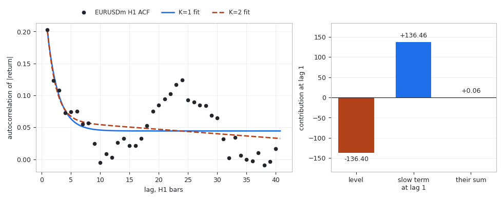
Fig. 8. The two curves are visually indistinguishable, and the second gets there by canceling two numbers hundreds of times larger than the data; both are refitted in Python to the points plotted here, so the magnitudes are the figure's own
That is what a degenerate fit looks like. A decay rate near zero over the fitted window is indistinguishable from a constant, so the level term and the slow exponential trade off along a flat valley and the solver stops wherever it runs out of progress. The two solvers stop 2544 apart in parameter space while agreeing on the sum of squares to five figures, 5.0717e-02 either way. Fitting the plotted points again in Python, which is what Fig. 8 draws, stops at a level of -136 instead of -2915: the same valley from a third starting point.
The AD Jacobian is exact; every entry agrees with the reverse mode Jacobian to 2.124e-16. It changes nothing here, because the problem is not that the derivative was approximate. The problem is that the model has a direction along which the data has no opinion, and no derivative, however exact, can supply an opinion the data does not hold.
Important: the curve above is 6000 EURUSDm H1 closes from 2025.09.18 08:00 to 2026.09.07 07:00 server time, read on 2026-09-07 at 07:46 GMT on an Exness demo account, server Exness-MT5Trial15, whose clock runs at GMT+0 and does not shift with daylight saving. The newest bar of that window was still forming when it was read. The script takes the newest bars rather than fixed dates, so a later run covers a later window. The half life of three million bars is not a measurement of the market. It is the fit reporting that it could not tell the slow term from the constant.
The practical reading is that an exact Jacobian buys speed and removes a tuning parameter. It does not buy identifiability, and a fit reporting an amplitude of 2915 on a curve bounded by 0.2 is pointing at the problem, not at the solver. Running that same fit a few hundred times, which is what the chart version below does, identifies what the problem actually is.
The same fit, running on a chart
The fitting script asks its question once, on the latest bars. A question asked a few hundred times gives up more. AD_ACFFit rebuilds the autocorrelation over a window ending at each bar, hands the same level plus two exponentials to the same solver with the same AD Jacobian, and plots what comes back.
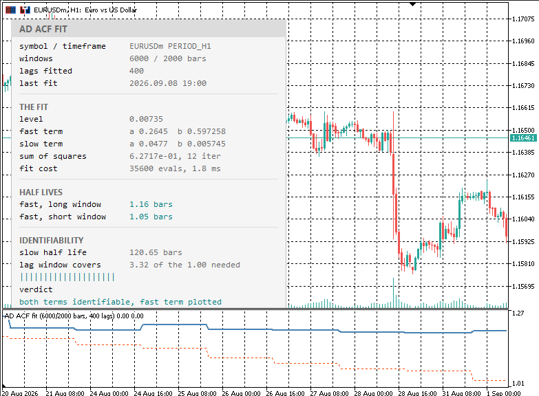
Fig. 9. The panel carries the last fit and the gate deciding whether it may be published; the subwindow carries the fast half life from a long and a short price window, flat between refits
The panel states what the fit was given, what came back, and whether the result is allowed on the chart at all. Here it returns a level of 0.00735, a fast term with amplitude 0.2645 and rate 0.597258, a slow term with amplitude 0.0477 and rate 0.005745, and a sum of squares of 6.2717e-01 after 12 iterations, at a cost of 35,600 residual evaluations and 1.8 milliseconds. The fast rate is a half life of 1.16 bars on the long window and the short window returns 1.05, and both are published because the 400 lag window covers 3.32 slow half lives against the one needed.
The model does not describe everything in the curve, and Fig. 8 shows what it misses: a bump peaking at lag 24, the daily volatility cycle on an H1 chart. A level plus two exponentials has no periodic component, so the fit runs through the middle of that seasonality rather than describing it.
Running the fit over many windows settles the question the previous section left open. The two term fit there was degenerate, and the reason was not the second exponential. It was the lag window. Forty lags is not enough of the curve for a slow decay to be told apart from a constant, and the fit stops being degenerate as soon as it is shown more.
| Lags | Largest amplitude | Fast half life | Slow half life | Slow half lives covered | Verdict |
|---|---|---|---|---|---|
| 40 | 3313 | 1.066 | 3,281,620 | 0.00 | not identifiable |
| 100 | 0.2584 | 1.225 | 32.05 | 3.12 | identifiable |
| 200 | 0.2621 | 1.160 | 111.82 | 1.79 | identifiable |
| 400 | 0.2614 | 1.173 | 121.24 | 3.30 | identifiable |
| 800 | 0.2631 | 1.140 | 102.02 | 7.84 | identifiable |
At 40 lags the largest amplitude is 3313 on a curve bounded by 0.2 and the slow half life is three million bars, so the window covers none of it. At 100 lags and beyond the amplitudes drop to about a quarter, both half lives are numbers the window can see, and the fit is well posed. The model was never over parameterized. It was under observed, the trap the synthetic fit avoids by choosing a spacing that resolves its slowest decay.
That is a criterion, not a judgment call, so the indicator applies it: a fit may publish a reading only if the solver returned one of ALGLIB's documented success codes, no amplitude is absurd against a curve bounded by one, and the lag window covers the slow term at least once. ALGLIB documents 1, 2 and 4 as its successes, while 5 means the iteration limit was reached, 7 that the solver stalled and -9 that its derivative check failed; the gate accepts the first three and refuses the rest.
//+------------------------------------------------------------------+
//| Fit the current autocorrelation and sort the result into a fast  |
//| and a slow term                                                  |
//|                                                                  |
//|  A decay the lag window cannot cover once is not distinguishable |
//|  from the constant term, so that case is marked rather than      |
//|  reported as a measurement.                                      |
//+------------------------------------------------------------------+
void FitCurrentACF(ACFFit &out)
  {
   g_K = 2;
   g_n = 5;
   g_resEval = 0;

//--- a start point with one clearly fast and one clearly slow rate, so
//--- the two terms do not begin life on top of each other
   double x[] = {0.0, 0.1, 0.05, 0.5, 0.01};

   CMinLMStateShell  state;
   CMinLMReportShell rep;

   ulong t0 = GetMicrosecondCount();
   CAlglib::MinLMCreateVJ(g_n, g_m, x, state);
   CAlglib::MinLMSetCond(state, 0.0, InpMaxIts);
   CAlglib::MinLMOptimize(state, g_fvec, g_jac, g_rep, false, g_obj);
   double p[];
   CAlglib::MinLMResults(state, p, rep);
   out.ms = (double)(GetMicrosecondCount() - t0) / 1000.0;

//--- ALGLIB documents 1, 2 and 4 as success. Code 5 is maxits, 7 a
//--- stalled solver and -9 a failed check: none of those may publish
   int term = rep.GetTerminationType();
   out.converged = (term == 1 || term == 2 || term == 4);
   out.iters     = rep.GetIterationsCount();
   out.resEval   = g_resEval;
   out.sse       = SSE(p);
   out.level     = p[0];

   int iFast = (p[3] >= p[4] ? 0 : 1);
   out.aFast = p[1 + iFast];
   out.bFast = p[3 + iFast];
   out.aSlow = p[2 - iFast];
   out.bSlow = p[4 - iFast];
   out.hlFast = (out.bFast > 0.0 ? MathLog(2.0) / out.bFast : -1.0);
   out.hlSlow = (out.bSlow > 0.0 ? MathLog(2.0) / out.bSlow : -1.0);
   out.covers = (out.hlSlow > 0.0 ? g_t[g_m - 1] / out.hlSlow : 0.0);

//--- a large amplitude paired with a rate near zero is a constant
//--- wearing an exponential's clothes, which the level already provides
   double bigA = MathMax(MathAbs(out.aFast), MathAbs(out.aSlow));
   out.identifiable = (out.converged && bigA <= 100.0 && out.covers >= 1.0);
  }
The last three lines are the whole test. Everything above them is the fit and the sorting of its two terms into a faster and a slower one, since Levenberg-Marquardt returns them in no particular order.
One reading survives that test and one does not. Holding the lag window at 400 and varying the bars the autocorrelation is measured over, the fast half life moves between 1.06 and 1.74 while the slow one runs from 32 to 849, and at 24,000 bars the slow term escapes the window and the fit is refused.
| Bars | Fast half life | Slow half life | Verdict |
|---|---|---|---|
| 1500 | 1.059 | 32.14 | identifiable |
| 2000 | 1.063 | 32.39 | identifiable |
| 3000 | 1.230 | 47.20 | identifiable |
| 4000 | 1.290 | 101.34 | identifiable |
| 6000 | 1.173 | 121.24 | identifiable |
| 12000 | 1.741 | 140.93 | identifiable |
| 24000 | 1.480 | 848.54 | not identifiable |
A quantity that grows with the data used to measure it is a property of the measurement, not of the market, and it is what fitting an exponential to a decay that is not exponential produces. So the indicator plots the fast half life, which survives a sixteen fold change in window inside a factor of two, and prints the slow one beside the window it came from rather than drawing it as though it meant something alone.
The plotting is deliberately unambitious. Refitting on every bar over any useful history is more work than a chart thread should do, so a refit happens every InpRefitEvery bars and each bar in between carries the most recent reading.
   int start;
   if(prev_calculated == 0)
     {
      ArrayInitialize(BufFastLong,  EMPTY_VALUE);
      ArrayInitialize(BufFastShort, EMPTY_VALUE);
      g_firstBar  = MathMax(need, rates_total - InpHistoryBars);
      g_nextFit   = g_firstBar;
      g_lastLong  = EMPTY_VALUE;
      g_lastShort = EMPTY_VALUE;
      g_haveFit   = false;
      start       = g_firstBar;
     }
   else
      start = MathMax(g_firstBar, prev_calculated - 1);

   bool refitted = false;
   for(int i = start; i <= last; i++)
     {
      if(i >= g_nextFit)
        {
         if(RefitAt(close, i))
           {
            g_fitTime = time[i];
            refitted  = true;
           }
         g_nextFit = i + MathMax(1, InpRefitEvery);
        }
      BufFastLong[i]  = g_lastLong;
      BufFastShort[i] = g_lastShort;
     }
//--- the forming bar has no reading of its own
   BufFastLong[rates_total - 1]  = EMPTY_VALUE;
   BufFastShort[rates_total - 1] = EMPTY_VALUE;
The forming bar is excluded on purpose and the history is bounded on purpose. One refit costs 45 to 55 milliseconds on EURUSDm H1, about four fifths of it the two fits rather than the two autocorrelations. The default 500 bars at one refit every 24 therefore costs roughly a second of chart thread on load, and nothing afterwards until a bar closes.
Important: a half life describes a fitted curve, not a forecast. Nothing here says a rising fast half life should be traded, and the indicator draws no signal. What it shows is a fit and the evidence for it, on data the reader can change under it.
The edges AD does not smooth over
Two limitations are inherent to the method rather than to this implementation, and the test script prints both rather than leaving them to be discovered.
//+------------------------------------------------------------------+
//| SECTION 5                                                        |
//|                                                                  |
//|  The honest edges. A tape records the branch that ran, absolute  |
//|  value has no derivative at zero, and both facts are printed     |
//|  here rather than left for a reader to discover.                 |
//+------------------------------------------------------------------+
void Section5_Edges(void)
  {
   Print("SECTION 5  where AD tells a partial truth");
   double grad[];

//--- f(x) = x for x > 0, else 2x. The kink at zero is real, and the
//--- tape can only ever describe the side it walked down
   double pts[] = {2.0, -2.0, 0.0};
   double wants[] = {1.0, 2.0, 2.0};
   for(int j = 0; j < 3; j++)
     {
      g_ADTape.Reset();
      ADVar x = ADInput(pts[j]);
      ADVar f = (pts[j] > 0.0 ? x * 1.0 : x * 2.0);
      g_ADTape.Gradient(f.slot, grad);
      PrintFormat("    branch at x=%+.1f gives slope %.1f (taken branch only)",
                  pts[j], grad[0]);
      Check(StringFormat("branch x=%+.1f", pts[j]), grad[0], wants[j], 1e-15);
     }
   Print("  at x=0 the two sides disagree; AD reports the branch that ran");

//--- |x| at zero, where the convention is stated rather than derived
   g_ADTape.Reset();
   ADVar z = ADInput(0.0);
   ADVar az = ADAbs(z);
   g_ADTape.Gradient(az.slot, grad);
   PrintFormat("    d|x|/dx at x=0 returns %.1f by convention, not by math",
               grad[0]);
   Check("abs at zero is the stated 0", grad[0], 0.0, 1e-15);

//--- a long loop, to show the tape is the thing that grows
   g_ADTape.Reset();
   ADVar acc = ADInput(1.0);
   for(int i = 0; i < 5000; i++)
      acc = acc * 1.0001;
   int nodes = g_ADTape.Count();
   g_ADTape.Gradient(acc.slot, grad);
   double want = MathPow(1.0001, 5000);
   PrintFormat("    5000 iterations recorded %d nodes", nodes);
   Check("5000 step chain rule", grad[0], want, 1e-12);
  }
The first is branching. A tape records the branch that actually ran, so the derivative you get is that of the path taken, not of the function as a whole. For a piecewise definition that is x above zero and 2x below, AD reports a slope of 1 at x=2 and 2 at x=-2, both correct. At x=0 the two sides genuinely disagree and AD reports whichever branch it was sent down. There is no derivative there, so reporting one is a convention.
The second is the absolute value at zero, which has the same shape. The code returns a sign of zero and the test asserts that value, making the convention part of the specification rather than an accident.
SECTION 5  where AD tells a partial truth
    branch at x=+2.0 gives slope 1.0 (taken branch only)
  [PASS] branch x=+2.0                      got 1  want 1  rel 0.000e+00
    branch at x=-2.0 gives slope 2.0 (taken branch only)
  [PASS] branch x=-2.0                      got 2  want 2  rel 0.000e+00
    branch at x=+0.0 gives slope 2.0 (taken branch only)
  [PASS] branch x=+0.0                      got 2  want 2  rel 0.000e+00
  at x=0 the two sides disagree; AD reports the branch that ran
    d|x|/dx at x=0 returns 0.0 by convention, not by math
  [PASS] abs at zero is the stated 0        got 0  want 0  rel 0.000e+00
    5000 iterations recorded 5001 nodes
  [PASS] 5000 step chain rule               got 1.6486800559310761  want 1.648680055931085  rel 5.387e-15
-----------------------------------------------------------
  worst analytic relative error : 2.878e-16
  worst forward vs reverse      : 2.878e-16
  21 passed, 0 failed
=== ALL PASS ===============================
The last case is about memory rather than mathematics. Five thousand multiplications record 5001 nodes and the chain rule composes across all of them, to 5.387e-15 against the closed form. But those nodes are real memory, and a loop long enough to be interesting is a tape long enough to matter. Reverse mode trades space for the single sweep, and on a long recording that trade is visible.
Two smaller cautions belong here. ADPow takes a constant exponent only, so a variable in the exponent has to be written as exp of a product. And the tape is a single global object, which keeps the overloads simple but allows one recording at a time: a function recording while another is open would interleave nodes on the same tape.
Conclusion
The library computes derivatives exact to within one or two units in the last place, in two modes, with no step size to choose anywhere. That claim is checked against closed forms, against the two modes compared with each other, and against jax at a tolerance derived from a measured floor rather than assumed. All 21 assertions in the test script pass, all 8 in the fitting script, and all 14 cross-check rows.
Three of the findings are worth carrying away more than the code is.
Forward mode fills a Jacobian column per sweep and reverse mode a row, and least squares has far more residuals than parameters, so forward mode does the fewer sweeps. On the clock it led at three of the four model sizes measured here and trailed at the fourth, which makes it the mode to reach for in this implementation rather than a rule that holds everywhere. Automatic differentiation is slower than finite differences below about five parameters and only pulls away past twenty, so the argument for it at small n is exactness rather than speed. And an exact Jacobian cannot make a parameter identifiable when the data does not reach far enough to constrain it: on 40 lags of real autocorrelation a two-exponential fit produces a level and an amplitude near 2915 that cancel to 0.06. Widening the window to 100 lags fixes that, which is the more useful half of the lesson.
Three types carry the library. ADDual is the forward mode dual number, costing one sweep per input. CADTape is the reverse mode tape, storing only parent slots and local partials, with capacity doubling and a single backward sweep whose cost is independent of the input count. ADVar is the recording type, carrying the same function set as the forward mode so a model can be written once and differentiated either way.
| # | Filename | Type | Description |
|---|---|---|---|
| 1 | ADTape.mqh | Include | The whole library: ADDual, CADTape, ADVar, and the elementary functions in both forms |
| 2 | AD_Test.mq5 | Script | 21 assertions: closed form derivatives, multi-parameter gradients, the step size sweep, cost against parameter count, and the branching edges |
| 3 | AD_Fit.mq5 | Script | 8 assertions: the AD Jacobian handed to ALGLIB's Levenberg-Marquardt, both modes against the numerical path, the diffstep sweep, and the real data fit |
| 4 | AD_Export.mq5 | Script | Writes seven functions, both modes, inputs and gradients at full precision to Common\Files\ad_gradients.csv for the Python cross-check |
| 5 | ad_crosscheck.py | Python | Differentiates the same seven functions with jax and compares in units in the last place, measuring the library floor first; run AD_Export.mq5 before it |
| 6 | AD_ACFFit.mq5 | Indicator | Runs the two-exponential fit on a rolling window with the AD Jacobian, plots the fast half life from a long and a short window, and reports the fit and its identifiability on a panel |
| 7 | MQL5.zip | Archive | Archive with all project files in their subfolders; unpack it into the terminal data directory and every file lands in its required location |
Warning: All rights to these materials are reserved by MetaQuotes Ltd. Copying or reprinting of these materials in whole or in part is prohibited.
This article was written by a user of the site and reflects their personal views. MetaQuotes Ltd is not responsible for the accuracy of the information presented, nor for any consequences resulting from the use of the solutions, strategies or recommendations described.


