Integrating MQL5 with data processing packages (Part 1): Advanced Data analysis and Statistical Processing

Introduction

Financial markets generate vast amount of data, which can be challenging to analyze for the sole purpose of technical analysis, well technical analysis alone done manually does not enable traders to analyze and interpret patterns, trends and anomalies within the data. Advanced data analysis package like Jupyter Lab allows traders to perform sophisticated statistical analysis, machine learning, and data visualization. This will aid in identifying profitable trading opportunities, understanding market behavior, seasonal tendencies, and predict future price movements.

Gather Historical data

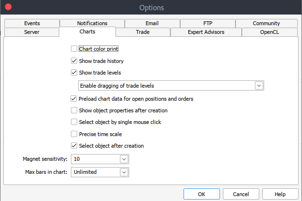
To get started we need historical data from MetaTrader 5 saved in .csv format, so simply launch your MetaTrader platform and at the top of your MetaTrader 5 pane/panel navigate to > Tools and then > Options and you will land to the Charts options. You will then have to select the amount of Bars in the chart you want to download. It's best to choose the option of unlimited bars since we'll be working with date and we wouldn't know how many bars are there in a given period of time.

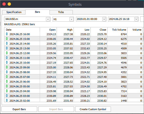
After that you will now have to download the actual data. To do that you will have to navigate to > View and then to  > Symbols and you will land on the Specifications tab simply navigate to > Bars or Ticks depending on what kind of data want to download. Proceed and enter the start and end date period of the historical data you want to download, after that click on the request button to download the data and save it in the .csv format.

After all those steps you would have successfully download historical data from your MetaTrader trading platform. Now you need to download and set up the Jupyter Lab environment for analysis. To download and set up Jupyter Lab you can head to their official website and follow simple step to download it. Depending on the type of operating system you use, you will have variety of options of whether to install using pip, conda or brew.

Load MetaTrader 5 Historical Data on Jupyter Lab

To successfully load your MetaTrader 5 historical data on Jupyter Lab you will have to know the folder that you had selected to download the data to, and then on Jupyter Lab simply navigate to that folder.To get started you will have to load the data and inspect the column names. We have to inspect the column names so that we handle the columns correctly and avoid errors that might arise if we use the wrong column name.

Preprocessing

Before we dive into data analysis, we need to preprocess the data.

1. Date-Time Parsing: Convert the date column into date-time format.

2. Missing value handling: Handle any missing values.

3. Feature Engineering: Create new features if necessary.

python code:

import pandas as pd

# Load historical data
file_path = '/home/int_junkie/Documents/ML/XAUUSD.m_H1_historical.csv'
data = pd.read_csv(file_path)

# Display the first few rows and column names
print(data.head())
print(data.columns)

output:

From the output we can see that there are some special characters '<>' within the columns and the presence of '\t' which indicates that the file is tab-separated now we can proceed to load historical data with the correct column name.

In the code below we'll be doing the following:

1. Importing libraries:

• Pandas is a powerful data manipulation library in Python.
• Technical Analysis Library (TA lib) is used for technical analysis of financial markets data.

2. Load historical data:

• File-path is used to specify the location of the CSV file containing historical data.
• Pd.read reads the CSV file into a pandas Data-Frame. The delimiter '\t' indicates that the file is tab-separated.

3. Displaying data:

• Data.head prints the first few rows of the Data-frame to verify the contents.
• Data.columns prints the column names to verify the structure of the data frame
  

4. Sorting data by date:

• Date.sort, sorts the data-frame in place based on the '<DATE>' column. This ensures the data is in chronological order.

5. Calculating RSI:

• TA.RSI calculates the Relative Strength Index (RSI) using the '<CLOSE>' price column.
• Time-period, specifies a 14-period RSI.
• The calculated values are stored in a new column named 'RSI' in the data frame.

6. Displaying the updated data:

• Data.head, prints the first few rows of the updated data-frame to verify the RSI calculation.

python code:

import pandas as pd
import talib as ta

# Load historical data
file_path = '/home/int_junkie/Documents/ML/XAUUSD.m_H1_historical.csv'
data = pd.read_csv(file_path, delimiter='\t')

# Display the first few rows and column names to verify
print(data.head())
print(data.columns)

# Ensure data is sorted by the correct date column
data.sort_values('<DATE>', inplace=True)

# Calculate RSI using the '<CLOSE>' price column
data['RSI'] = ta.RSI(data['<CLOSE>'], timeperiod=14)

# Display the first few rows to verify
print(data.head())

output:

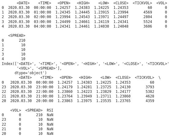
From the output we can see that we have NAN values under the RSI column, we have to handle the NAN values correctly. The RSI function requires a minimum number of data points to calculate the indicator. It might return NAN values for initial periods. To handle the NAN values correctly we need to know the data type for column '<CLOSE>'. Ensure that the Data-Frame and column access is correct. The following python code show how to handle the NAN values.

import pandas as pd
import talib as ta

# Load the historical data
file_path = '/home/int_junkie/Documents/ML/XAUUSD.m_H1_historical.csv'
data = pd.read_csv(file_path, delimiter='\t')data['<CLOSE>'] = data['<CLOSE>'].astype(float)


# Verify the column names
print(data.columns)

# Convert the column to the correct data type if necessary
data['<CLOSE>'] = data['<CLOSE>'].astype(float)

# Calculate the RSI
data['RSI'] = ta.RSI(data['<CLOSE>'], timeperiod=14)

# Display the RSI values
print(data[['<CLOSE>', 'RSI']].tail(20))

Output:

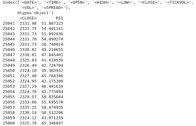
We can see that we have correctly handled the NAN values. If you see a NAN value for the initial periods (which is expected due to the lock-back period), you can proceed to handle them as follows:

data['RSI'] = ta.RSI(data['<CLOSE>'], timeperiod=14)
data['RSI'] = data['RSI'].fillna(0)  # or use any other method to handle NaN values

Exploratory Data Analysis

EDA's main goal is to understand the underlying structure of the data, by summarizing the main characteristics of the data. When performing EDA we discover patterns and identify trends and relationship within the data. In EDA we also detect anomalies and outliers or any unusual observations that may need further investigation. We also check assumptions about the data that might affect subsequent analysis. We then perform data cleaning by looking for any missing values, errors, inconsistencies in the data that need to be addressed. 

We use the following python scripts to perform EDA:

import seaborn as sns
import matplotlib.pyplot as plt
import warnings

warnings.filterwarnings("ignore")

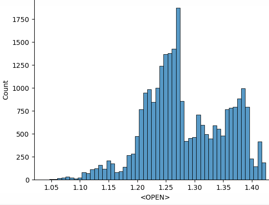
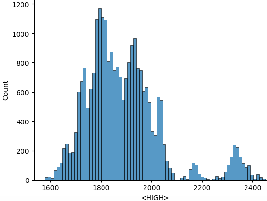
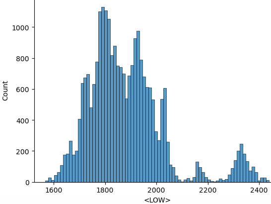
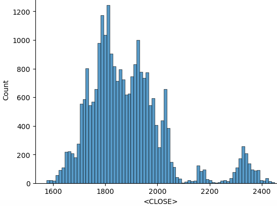
for i in data.select_dtypes(include="number").columns:
    sns.histplot(data=data, x=i)
    plt.show()

From the code above after importing all the necessary libraries we start by ignoring the warnings in order to get clean output. We then iterate through the numerical columns, and ' data.select_dtypes(include="number")'   returns the data frame containing only the numerical columns and 'columns' returns the names of these columns. And then proceed to plot the histogram from the data. Here are the histograms plotted from the code above.

   

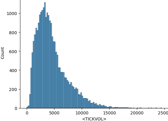
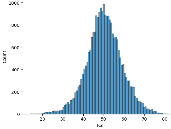
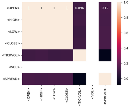
After the operations of statistical processing, we can proceed to train the model on the gathered data. The goal is to be able to make predictions from the historical data that we gathered. We are going to make predictions using only RSI indicator. Before doing the we need to know the kind of relationship that exits between the data itself, we do that by performing the correlation matrix. We should be able to interpret whether the relationship that exist has positive correlation, negative correlation, or no correlation.

• Positive correlation: Values close to 1 indicate a strong positive correlation between two variables. For example, if the correlation between 'Open' and 'Close' is close to 1, it means they move in the same direction.
• Negative correlation: Values close to -1 indicate a strong negative correlation. For example, if the correlation between 'Volume' and 'Price' is close to -1, it means that as the volume increases, the price tends to decrease.
• No correlation: Values close to 0 indicate no correlation between the variables.

import pandas as pd
import numpy as np
import matplotlib.pyplot as plt
import seaborn as sns
from sklearn.model_selection import train_test_split
from sklearn.ensemble import RandomForestRegressor
from sklearn.metrics import r2_score, mean_squared_error
import talib as ta  # Technical Analysis library

# Load the data
file_path = '/home/int_junkie/Documents/ML/XAUUSD.m_H1_historical.csv'
data = pd.read_csv(file_path, delimiter='\t')

# Exploratory Data Analysis (EDA)
print(data.info())
print(data.describe())

# Visualize the closing price
plt.figure(figsize=(12, 6))
plt.plot(data['<CLOSE>'])
plt.title('XAUUSD Closing Price')
plt.xlabel('<DATE>')
plt.ylabel('Price')
plt.show()

# Feature Engineering
data['RSI'] = ta.RSI(data['<CLOSE>'], timeperiod=14)

# Drop rows with missing values
data.dropna(inplace=True)

# Define target variable
data['Target'] = data['<CLOSE>'].shift(-1)
data.dropna(inplace=True)

# Split the data
X = data[['RSI']]  # Only use RSI as the feature
y = data['Target']

X_train, X_test, y_train, y_test = train_test_split(X, y, test_size=0.2, shuffle=False)

# Model Development
model = RandomForestRegressor(n_estimators=100, random_state=42)
model.fit(X_train, y_train)

# Predictions
y_pred = model.predict(X_test)

# Evaluate the model
mse = mean_squared_error(y_test, y_pred)
print(f'Mean Squared Error: {mse}')

# Visualize the predictions
plt.figure(figsize=(12, 6))
plt.plot(y_test.index, y_test, label='Actual Values')
plt.plot(y_test.index, y_pred, label='Predicted Values')
plt.xlabel('Samples')
plt.ylabel('TARGET_CLOSE')
plt.title('Actual vs Predicted Values')
plt.legend()
plt.show()

This is the output we get when training the model:

 

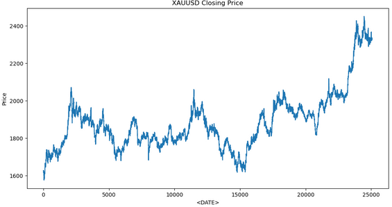
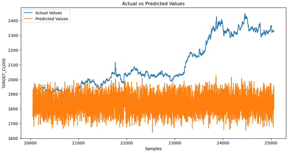
Although from the data analysis we can see that the predicted values do not match the actual values. This indicates that the model is not capturing the underlying pattern effectively. Several factors could contribute to this.

1. Insufficient training data: If the data set is too small, the model might not have enough information to learn meaning full information.

2. Overfitting: The model may have memorized the learning data rather than learning to generalize from it. This often when the model is too complex or not generalized properly.

3. Underfitting: The model may be too simple to capture the underlying pattern in the data. This can happen if the model doesn't have enough enough complexity or if important features are missing.

4. Feature Engineering: Poor feature selection or insufficient engineering can result in the model not having enough relevant information to make predictions.

Steps to diagnose and fix the issue:

1. Check the data: Ensure data is clean, consistent, and properly preprocessed.

2. Evaluate model performance: Use matrix such as Mean Squared Error (MSE), and Mean Absolute Error (MAB).

3. Improve feature engineering: Experiment with different features, including technical indicators, lagged values, and other relevant financial metrics.

4. Tune Hyper-parameters: Use techniques like Grid Search or Random Search to find optimal hyper-parameter for your model.

Putting it all together on MQL5

After saving the model, we then need to create a python script for predictions. This script will load the model and make predictions.

import joblib
import sys
import os

• Joblib: Is used to load the serialized machine learning model.
• Sys: Which is short for 'system', provides access to command-line arguments.
• OS: Which is short for 'Operating System', is used to check the existence of files and perform file operations.

model_path = sys.argv[/home/int_junkie/Documents/ML/random_forest_model.pkl]
features_path = sys.argv[/home/int_junkie/Documents/ML/features.txt]

• Sys.argv[1]: The first command-line argument, is the path to the model file.
• Sys.argv[2]: The second command-line argument, is the path to the features file.

print(f"Model path: {model_path}")
print(f"Features path: {features_path}")

Printing debugging information. Prints the paths of the model and features files for debugging purposes.

if not os.path.exists(model_path):
    print(f"Error: Model file not found at {model_path}")
    sys.exit(1)

if not os.path.exists(features_path):
    print(f"Error: Features file not found at {features_path}")
    sys.exit(1)

• Checks if the model file and features file exists.
• If either does not exist, prints an error message and exits the script with a status code of 1.

model = joblib.load(model_path)

• Loads the trained machine learning model from the specified 'model-path'.

with open(features_path, 'r') as f:
    features = [float(line.strip()) for line in f]

• Opens the features file for reading.
• Reads each line, strips any leading/trailing white-spaces, converts the file to a float, and stores it in the 'features' list.

prediction = model.predict([features])[0]

• Uses the loaded model to make a prediction based on the loaded features.
• Model.predict: Returns a list of predictions (in this case a single prediction), and '[0]' extracts the first prediction.

print(prediction)

• Prints the prediction to a strand output. This output can be captured by another script or program, such as MQL5, to make trading decisions.

MQL5

Load the model on the OnInit().

int OnInit(){
   // Load the model and feature names
   string modelPath = "/home/int_junkie/Documents/ML/random_forest_model.pkl";
   string featurePath = "/home/int_junkie/Documents/ML/features.txt";
   
   // Your code to load the model (use appropriate library for pkl files)

   // Initialize the features
   double features[];
   int fileHandle = FileOpen(featurePath, FILE_READ | FILE_TXT);
   if (fileHandle != INVALID_HANDLE)
     {
      string line;
      while(!FileIsEnding(fileHandle))
        {
         line = FileReadString(fileHandle);
         ArrayResize(features, ArraySize(features) + 1);
         features[ArraySize(features) - 1] = StringToDouble(line);
        }
      FileClose(fileHandle);
     }

   return(INIT_SUCCEEDED);
  }

Reading the predictions from the python file on the OnTick().

void OnTick(){
   // Declare static variables to retain values across function calls
   static bool isNewBar = false;
   static int prevBars = 0;
   
   // Get the current number of bars
   int newbar = iBars(_Symbol, _Period);
   
   // Check if the number of bars has changed
   if (prevBars == newbar) {
       // No new bar
       isNewBar = false;
   } else {
       // New bar detected
       isNewBar = true;
       // Update previous bars count to current
       prevBars = newbar;
   }
   
   // Update the features based on current data
   double features[];
   ArrayResize(features, 1);
   features[0] = iClose(Symbol(), 0, 0);
   
   // Write the features to a file
   int fileHandle = FileOpen("/home/int_junkie/Documents/ML/features.txt", FILE_WRITE | FILE_TXT);
   if (fileHandle != INVALID_HANDLE)
     {
      for (int i = 0; i < ArraySize(features); i++)
        {
         FileWrite(fileHandle, DoubleToString(features[i]));
        }
      FileClose(fileHandle);
     }
   else
     {
      Print("Error: Cannot open features file for writing");
      return;
     }
     
      // Call the Python script to get the prediction
   string command = "python /home/int_junkie/Documents/ML/predict.py /home/int_junkie/Documents/ML/random_forest_model.pkl /home/int_junkie/Documents/ML/features.txt";
   int result = ShellExecuteA(command);
   if(result != 0)
     {
      Print("Error: ShellExecuteA failed with code ", result);
      return;
     }

   // Read the prediction from a file
   Sleep(1000); // Wait for the Python script to complete
   fileHandle = FileOpen("/home/int_junkie/Documents/ML/prediction.txt", FILE_READ | FILE_TXT);
   if (fileHandle != INVALID_HANDLE)
     {
      string prediction = FileReadString(fileHandle);
      FileClose(fileHandle);

      double pred_value = StringToDouble(prediction);

      // Generate trading signals based on predictions
      double some_threshold = 0.0; // Define your threshold
      if (pred_value > some_threshold)
        {
         // Buy signal
         double Ask = NormalizeDouble(SymbolInfoDouble(_Symbol,SYMBOL_ASK),Digits());
         double sl =  Ask - stopLoss * _Point;
         double tp =  Ask + takeProfit * _Point;
         trade.PositionOpen(_Symbol, ORDER_TYPE_BUY, lotsize, Ask, sl, tp, "ML");
        }
      else if (pred_value < some_threshold)
        {
         // Sell signal
         double Bid = NormalizeDouble(SymbolInfoDouble(_Symbol,SYMBOL_BID),Digits());
         double sl = Bid + stopLoss * _Point;
         double tp = Bid - takeProfit * _Point;
         trade.PositionOpen(_Symbol, ORDER_TYPE_SELL, lotsize, Bid, sl, tp, "ML");
        }
     }
   else
     {
      Print("Error: Cannot open prediction file for reading");
     }
  }

On the OnTick the variable 'command' prepares a string command to run a python script with a feature file and model file as arguments. ShellExecuteA (command) executes the python script using ShellExecuteA. 'Sleep (1000)', Waits for 1 second the python script completes execution. After that we open the prediction file for reading. We then check if the prediction file opened successfully. If yes, reads the prediction. If no, prints an error. The threshold variable is used to make trading decisions. If it's greater than the predicted value, generates a buy signal. If it's lesser than the predicted value, generates a sell signal.

Conclusion

In summary, we have gathered data from MetaTrader 5 trading platform. The same date that we gathered we then use it in Jupyter Lab to perform data analysis and statistical processing. After performing the analysis in Jupyter Lab, we then use the model and integrate it on MQL5 to make trading decisions from the identified patterns. Integrating MQL5 with Jupyter Lab solves the problem of limited analytical, statistical, and visualization capabilities in MQL5. The process enhances strategy development, improves data handling efficiency, and provides collaborative, flexible, and powerful environment for advanced data analysis and statistical processing in trading.

In conclusion, by integrating MQL5 with Jupyter Lab we can perform advanced data analysis and statistical processing. With such capabilities you can develop any kind of trading strategy, and optimize trading strategies with advanced techniques. As a result, it provides significant competitive edge in the dynamic and data intensive field of financial trading.