The Hilbert Spectrum in MQL5 — Live Time-Frequency-Energy Visualization of Market Cycles

Introduction

Look closely at almost any price chart and you will usually find more than one cycle running underneath it. A five-minute XAUUSD chart can carry a fast scalping-speed oscillation, a slower intraday swing, and an even slower multi-day drift, all stacked on top of each other and disguised as a single jagged line. Traditional tools force you to pick one lens at a time: a short moving average shows you the fast wiggle but hides the slow one, a long moving average does the opposite. What if you could see all of the cycles at once, watch their frequencies and energy shift in real time, and catch the moment a market rotates from a choppy, high-frequency regime into a smooth, low-frequency trend?

That is exactly what the Hilbert Spectrum gives you. It comes from the Hilbert-Huang Transform (HHT), which has two parts: Empirical Mode Decomposition (EMD), which peels a signal apart into a handful of oscillatory components without assuming any fixed basis functions the way Fourier analysis does, and Hilbert Spectral Analysis (HSA), which converts each of those components into an instantaneous frequency and energy reading at every bar. Stack those readings up over a rolling window and you get a live time-frequency-energy surface - the Hilbert Spectrum - painted directly on your chart.

Scope note: this article builds a diagnostic MQL5 indicator, not a signal-generating Expert Advisor. There is no trade execution logic here. The goal is to give you a live, on-chart lens into which cycles are dominating price right now, which you can then combine with your own entry/exit logic. All balance-curve style backtest figures are absent by design - what you get instead is numerical validation against a synthetic signal with known frequency content, plus a live rendering check on XAUUSD M5.

We will build this in MQL5 from the ground up. The pipeline covers four pieces: the sifting algorithm behind EMD, a windowed-FIR approximation of the discrete Hilbert transform (MQL5 has no native FFT-based analytic-signal call), instantaneous frequency extraction via phase unwrapping, and a CCanvas-based heatmap renderer that updates live as new bars form. Every function that does real work in this pipeline - from the spline envelope solver through the bar-close orchestration in OnCalculate() - is shown and explained below, not just referenced. Suggested MQL5 Community category for this piece is Indicators, since the deliverable is a custom indicator with an embedded visualization engine and zero trade management code.

A quick note on who this is for: you do not need a signal-processing background to follow along, but you do need to be comfortable reading MQL5 array code and willing to sit with a few formulas - the article walks through what each one means and why it is there before showing the code that implements it. If you already know EMD and the Hilbert-Huang Transform from another language, most of this will read as a straight port; if you have never touched either, the sifting-algorithm section below is written to stand on its own.

Why Time-Frequency Analysis, and How the Pieces Fit Together

Fourier analysis is the obvious first tool anyone reaches for when they want to talk about "frequency" in a price series. The catch is that a Fourier transform represents the whole window with a fixed set of sine and cosine waves chosen in advance, which forces a stationarity assumption onto financial data - the implicit premise that the frequency content doesn't meaningfully change over the window. Market cycles rarely cooperate: a gold rally accelerates and decelerates, swings get sharper near news events, and the dominant cycle length itself drifts over the session. Empirical Mode Decomposition takes a different approach - it is fully data-driven, extracting oscillatory modes directly from the local maxima and minima of the series itself rather than projecting onto a fixed basis, though that adaptivity brings its own tradeoffs (more on those in the Limitations section near the end).

The full pipeline looks like this: raw price comes in, EMD sifts it into a small number of Intrinsic Mode Functions (IMFs) ordered from fastest to slowest, each IMF is passed through a discrete Hilbert transform to build its analytic signal, and from that analytic signal we read off instantaneous amplitude and instantaneous frequency at every bar. Those (time, frequency, energy) triplets from every IMF get binned into a 2D matrix and rendered as a heatmap that updates live.

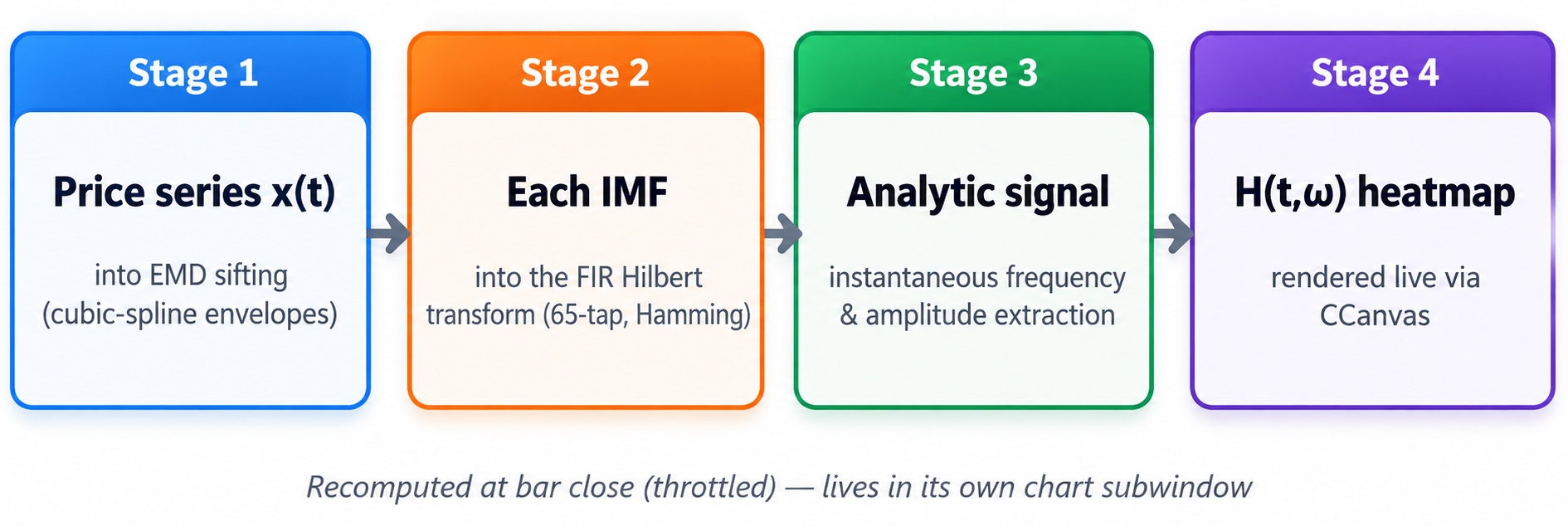
Fig. 1. The four-stage pipeline: price series into EMD sifting, each resulting IMF into the FIR Hilbert transform, instantaneous frequency and amplitude extraction, and finally the live H(t,ω) heatmap rendered through CCanvas.

One architectural decision worth flagging upfront: this is deliberately built as a diagnostic overlay, not embedded inside a strategy's OnTick(). Sifting is iterative and not cheap, so the indicator throttles recomputation to bar-close by default (configurable), and the whole thing lives in its own chart subwindow so it never interferes with your price action or other indicators.

It's worth addressing the obvious alternative: wavelet transforms also give you a time-frequency view, and MQL5 developers occasionally reach for them instead. The tradeoff is that a wavelet decomposition still requires you to pick a mother wavelet and a fixed dyadic scale ladder upfront, which reintroduces a basis-function assumption through the back door - just a more flexible one than a single sine wave. EMD's adaptivity is exactly what makes it attractive for price data with an unknown, time-varying number of dominant cycles: it discovers the number and shape of the oscillatory modes from the series itself rather than from a family of wavelets you chose in advance. The cost is sifting's iterative, per-window computation, which is the main reason this implementation throttles to bar close rather than recomputing on every tick.

In practical terms, here is how you actually read the finished panel: watch for a horizontal band splitting into two. That can mean a previously dominant cycle is genuinely fragmenting into faster and slower components - though it can also just be EMD re-partitioning the same underlying move slightly differently as the rolling window slides. Treat a single split or merge as a prompt to look closer, not as a confirmed regime change. A band's vertical position tells you the cycle length that is currently dominating, and its color (via the energy colormap covered later) tells you how energetic that cell is relative to the single hottest cell in the current window, not what share of the window's total energy it represents. None of that replaces your own entry and exit logic - it is a read on which timescale to even be paying attention to right now.

Empirical Mode Decomposition: the Sifting Algorithm

EMD works on a simple, almost mechanical idea. Take the price series x(t). Find every local maximum and connect them with a smooth interpolating curve to get an upper envelope e max (t). Do the same for the local minima to get a lower envelope e min (t). Average the two envelopes to get a local mean m(t) = (e max (t) + e min (t)) / 2, and subtract it from the series:

h(t) = x(t) - m(t)

In the formal definition, h(t) qualifies as an Intrinsic Mode Function once it satisfies two conditions: the number of extrema and the number of zero-crossings differ by at most one, and the mean of its upper and lower envelopes is close to zero everywhere. Checking both of those exactly on every single iteration is expensive and rarely done in practice, including here - this implementation leans on the extrema-count guard shown below (too few extrema to build an envelope from at all) plus the classic Cauchy-type standard-deviation criterion from Huang et al. (1998) as a converged-enough proxy for the second condition, computed between two consecutive sifting iterations k-1 and k:

SD = Σt [h(k-1)(t) - h(k)(t)]² / Σt h(k-1)(t)²

Sifting stops once SD drops below a threshold (0.25 in this implementation, inside the 0.2-0.3 range the original paper recommends). Once IMF 1 is extracted, it is subtracted from the original series to leave a residual, and the entire sifting loop is applied again to the residual to extract IMF 2, and so on, until the residual itself becomes essentially monotonic (fewer than three extrema) or a maximum IMF count is reached. Envelope interpolation uses a natural cubic spline - implemented from scratch in MQL5 via a Thomas-algorithm tri-diagonal solve for the spline's second derivatives, since MQL5 has no built-in spline interpolation function for irregularly spaced knots. Below is the full sifting pass, unabridged: it finds the extrema, guards against the degenerate case where a window has too few of them to build an envelope from, builds both envelopes via a spline-interpolation helper, and subtracts their local mean from the input.

SiftOnce

//+------------------------------------------------------------------+
//|      One sifting pass: upper/lower envelopes -> mean -> subtract |
//+------------------------------------------------------------------+
bool CEMD::SiftOnce(const double &h[],int count,double &next[],bool &degenerate)
  {
   int maxIdx[],minIdx[];
   FindExtrema(h,count,maxIdx,minIdx);
   degenerate=false;

   if(ArraySize(maxIdx)<HS_MIN_EXTREMA || ArraySize(minIdx)<HS_MIN_EXTREMA)
     {
      degenerate=true;
      ArrayResize(next,count);
      ArrayCopy(next,h);
      return(false);
     }

   double upper[],lower[];
   double maxVal[],minVal[];
   ArrayResize(maxVal,ArraySize(maxIdx));
   ArrayResize(minVal,ArraySize(minIdx));
   for(int i=0;i<ArraySize(maxIdx);i++) maxVal[i]=h[maxIdx[i]];
   for(int i=0;i<ArraySize(minIdx);i++) minVal[i]=h[minIdx[i]];

   SplineEnvelope(maxIdx,maxVal,ArraySize(maxIdx),count,upper);
   SplineEnvelope(minIdx,minVal,ArraySize(minIdx),count,lower);

   ArrayResize(next,count);
   for(int i=0;i<count;i++)
      next[i]=h[i]-0.5*(upper[i]+lower[i]);

   return(true);
  }

The degenerate guard on lines 10-16 matters more than it looks: without it, a flat or strongly one-directional stretch of price (fewer than HS_MIN_EXTREMA highs or lows) would leave the spline solver trying to interpolate through almost no points, which is exactly the kind of edge case that produces silent garbage in a live indicator rather than a clean failure. Here it just passes the input straight through and reports back that nothing changed, so the outer loop can decide to stop. Finding those extrema in the first place is a plain 3-point comparison scan - no interpolation, just a check against each sample's immediate neighbors:

FindExtrema

//+------------------------------------------------------------------+
//|   Find local maxima / minima indices (simple 3-point comparison) |
//+------------------------------------------------------------------+
void CEMD::FindExtrema(const double &series[],int count,int &maxIdx[],int &minIdx[])
  {
   ArrayResize(maxIdx,0);
   ArrayResize(minIdx,0);
   for(int i=1;i<count-1;i++)
     {
      if(series[i]>series[i-1] && series[i]>series[i+1])
        {
         int n=ArraySize(maxIdx);
         ArrayResize(maxIdx,n+1);
         maxIdx[n]=i;
        }
      else if(series[i]<series[i-1] && series[i]<series[i+1])
        {
         int n=ArraySize(minIdx);
         ArrayResize(minIdx,n+1);
         minIdx[n]=i;
        }
     }
  }

Before that outer loop, though, it's worth closing the loop on SiftOnce() itself: line 8's call to SplineEnvelope() is what actually builds the upper and lower envelopes from the extrema found above. It evaluates a natural cubic spline through the extrema at every integer bar position, holding flat before the first knot and after the last one:

SplineEnvelope

//+------------------------------------------------------------------+
//|    Evaluate the natural cubic spline over every integer position |
//|        0..count-1, extrapolating flat beyond the first/last knot |
//+------------------------------------------------------------------+
void CEMD::SplineEnvelope(const int &x[],const double &y[],int n,int count,double &envelope[])
  {
   ArrayResize(envelope,count);
   if(n==0)
     {
      ArrayInitialize(envelope,0.0);
      return;
     }
   if(n==1)
     {
      for(int i=0;i<count;i++) envelope[i]=y[0];
      return;
     }
   double y2[];
   SplineSecondDerivatives(x,y,n,y2);

   int seg=0;
   for(int i=0;i<count;i++)
     {
      if(i<x[0]) { envelope[i]=y[0]; continue; }
      if(i>x[n-1]) { envelope[i]=y[n-1]; continue; }
      while(seg<n-2 && i>x[seg+1]) seg++;
      double x0=x[seg], x1=x[seg+1];
      double h=x1-x0;
      if(h<=0) { envelope[i]=y[seg]; continue; }
      double a=(x1-i)/h;
      double b=(i-x0)/h;
      envelope[i]=a*y[seg]+b*y[seg+1]+
                  ((a*a*a-a)*y2[seg]+(b*b*b-b)*y2[seg+1])*(h*h)/6.0;
     }
  }

The spline itself needs second derivatives at each knot before it can be evaluated, and getting those from an arbitrary set of unevenly spaced knots is a tri-diagonal linear system - solved here with a direct Thomas-algorithm sweep rather than a general-purpose solver, since MQL5 has nothing built in for irregular-knot spline interpolation and a tri-diagonal system is cheap to solve directly:

SplineSecondDerivatives

//+------------------------------------------------------------------+
//|     Thomas algorithm tri-diagonal solve for natural cubic spline |
//|second derivatives at the knot points (x are strictly increasing) |
//+------------------------------------------------------------------+
void CEMD::SplineSecondDerivatives(const int &x[],const double &y[],int n,double &y2[])
  {
   ArrayResize(y2,n);
   if(n<3)
     {
      ArrayInitialize(y2,0.0);
      return;
     }
   double u[];
   ArrayResize(u,n);
   y2[0]=0.0;
   u[0]=0.0;
   for(int i=1;i<n-1;i++)
     {
      double sig=(double)(x[i]-x[i-1])/(double)(x[i+1]-x[i-1]);
      double p=sig*y2[i-1]+2.0;
      y2[i]=(sig-1.0)/p;
      double d1=(y[i+1]-y[i])/(double)(x[i+1]-x[i]);
      double d2=(y[i]-y[i-1])/(double)(x[i]-x[i-1]);
      u[i]=(6.0*(d1-d2)/(double)(x[i+1]-x[i-1])-sig*u[i-1])/p;
     }
   y2[n-1]=0.0;
   for(int k=n-2;k>=0;k--)
      y2[k]=y2[k]*y2[k+1]+u[k];
  }

That outer loop lives in Decompose(), which is the method the indicator actually calls once per redraw. It repeatedly hands the current residual to SiftOnce(), checks the Cauchy SD criterion after every pass, and once a mode stabilizes it stores that mode as the next IMF, subtracts it from the residual, and checks whether the residual itself still has enough extrema to keep going:

Decompose

//+------------------------------------------------------------------+
//|    Full decomposition: repeatedly extract IMFs from the residual |
//|  until the residual is monotonic/degenerate or m_maxImfs reached |
//+------------------------------------------------------------------+
int CEMD::Decompose(const double &price[],int count,double &imfs[][HS_MAX_LOOKBACK],double &residual[])
  {
   if(count<8) return(-1);
   if(count>HS_MAX_LOOKBACK)
     {
      Print("CEMD::Decompose - count (",count,") exceeds HS_MAX_LOOKBACK (",HS_MAX_LOOKBACK,")");
      return(-1);
     }

   ArrayResize(residual,count);
   ArrayCopy(residual,price);

   int extracted=0;
   for(int k=0;k<m_maxImfs;k++)
     {
      double h[];
      ArrayResize(h,count);
      ArrayCopy(h,residual);

      bool degenerateExit=false;
      for(int iter=0;iter<HS_SIFT_MAX_ITER;iter++)
        {
         double next[];
         bool degenerate=false;
         bool ok=SiftOnce(h,count,next,degenerate);
         if(!ok || degenerate)
           {
            //--- too few extrema to keep sifting: what's left is residual/
            //--- trend, not an oscillatory mode. Do not store it as an IMF.
            degenerateExit=true;
            break;
           }
         double sd=SDCriterion(h,next,count);
         ArrayCopy(h,next);
         if(sd<HS_SIFT_SD_THRESH)
            break;
        }

      //--- a degenerate stop means this k has no valid mode to contribute:
      //--- stop extracting altogether and leave the remainder in residual
      //--- rather than mislabeling a trend segment as an IMF
      if(degenerateExit)
         break;

      //--- store the extracted IMF (element-by-element: MQL5 does not support
      //--- row-slicing a fixed-second-dimension 2D array via ArrayCopy)
      for(int i=0;i<count;i++)
         imfs[k][i]=h[i];
      extracted++;

      //--- update residual
      for(int i=0;i<count;i++)
         residual[i]=residual[i]-h[i];

      //--- check if residual itself has too few extrema left -> stop extracting further IMFs
      int rMax[],rMin[];
      FindExtrema(residual,count,rMax,rMin);
      if(ArraySize(rMax)<HS_MIN_EXTREMA || ArraySize(rMin)<HS_MIN_EXTREMA)
         break;
     }

   return(extracted);
  }

The Cauchy SD check on line 37 is a direct implementation of the formula given earlier - sum the squared difference between consecutive sifting iterations, divide by the sum of squares of the previous iteration, and compare against the threshold:

SDCriterion

//+------------------------------------------------------------------+
//|    Cauchy-type SD stopping criterion between two sift iterations |
//+------------------------------------------------------------------+
double CEMD::SDCriterion(const double &prev[],const double &curr[],int count)
  {
   double num=0.0,den=0.0;
   for(int i=0;i<count;i++)
     {
      double diff=prev[i]-curr[i];
      num+=diff*diff;
      den+=prev[i]*prev[i];
     }
   if(den<=1e-12) return(0.0);
   return(num/den);
  }

Two safety rails matter here. HS_MAX_LOOKBACK bounds how large a window Decompose() will ever process, since the IMF storage array is a fixed-size compile-time array (MQL5's multidimensional array rules require a constant trailing dimension) - passing a longer window than that is rejected outright rather than silently truncated. And HS_SIFT_MAX_ITER caps the inner sifting loop per IMF, so a pathological window that never satisfies the SD threshold still terminates deterministically instead of hanging the chart.

On a synthetic signal built from two known sine waves plus a slow drift and a small amount of noise, this sifting loop cleanly separates the components back out. The fast 8-bar-period cycle lands in IMF1, the 34-bar-period cycle lands in IMF2, and the slow drift is absorbed into the residual - exactly the ordering EMD is supposed to produce, fastest oscillation first.

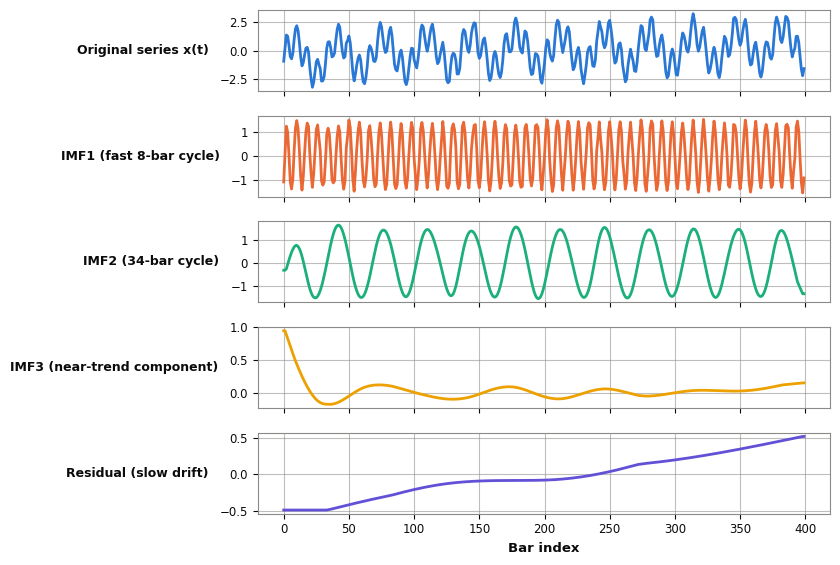
Fig. 2. Sifting output on a synthetic signal: original series, IMF1 (fast 8-bar cycle), IMF2 (34-bar cycle), IMF3 (near-trend component), and the residual. Each mode isolates a distinct oscillatory scale.

From IMFs to the Analytic Signal: the Discrete Hilbert Transform

An IMF on its own is just an oscillating number series - it doesn't hand you a frequency or an energy reading directly. To get those, you build the analytic signal z(t) = x(t) + i·y(t), where y(t) is the Hilbert transform of x(t). The ideal continuous Hilbert transform has kernel 1/(πt); its discrete equivalent is h[n] = 2/(πn) for odd n and zero for even n (including n=0). That kernel has infinite support, so in practice you truncate it to a finite number of taps and apply a window function to control the resulting passband ripple versus transition-bandwidth tradeoff. This implementation uses a 65-tap kernel with a Hamming window, built once in BuildKernel() and reused for every IMF:

BuildKernel

// Windowed-ideal-response FIR Hilbert kernel (odd taps only, Hamming-windowed)
void CHilbertTransform::BuildKernel(void)
  {
   ArrayResize(m_kernel,m_taps);
   int half=m_taps/2;
   for(int i=0;i<m_taps;i++)
     {
      int n=i-half;
      double ideal=0.0;
      if(n!=0 && n%2!=0)
         ideal=2.0/(M_PI*n);
      double w=0.54-0.46*MathCos(2.0*M_PI*i/(m_taps-1));
      m_kernel[i]=ideal*w;
     }
  }

Building the kernel is a one-time cost; applying it is the part that runs on every IMF, every redraw. Quadrature() convolves the input series directly against that kernel - a plain direct-form convolution rather than an FFT-based one, since a 65-tap kernel against a 200-bar window is cheap enough that the extra complexity of an FFT convolution buys nothing here. Samples that fall outside the window at either edge are treated as zero, which is exactly the assumption that produces the edge transients discussed further down:

Quadrature

//+------------------------------------------------------------------+
//|                Direct-form convolution, zero-padded at the edges |
//+------------------------------------------------------------------+
void CHilbertTransform::Quadrature(const double &series[],int count,double &quad[])
  {
   ArrayResize(quad,count);
   int half=m_taps/2;
   for(int n=0;n<count;n++)
     {
      double acc=0.0;
      for(int k=0;k<m_taps;k++)
        {
         int idx=n-(k-half);
         if(idx>=0 && idx<count)
            acc+=m_kernel[k]*series[idx];
        }
      quad[n]=acc;
     }
  }

Once you have the quadrature component y(t) from that convolution, instantaneous amplitude and phase fall out directly:

a(t) = √(x(t)² + y(t)²)    φ(t) = atan2(y(t), x(t))

Those two formulas map onto two small, single-purpose methods - deliberately kept separate rather than folded into one function, since the spectrum builder needs amplitude and phase at different points in its own pipeline:

InstantAmplitude

//+------------------------------------------------------------------+
//|              Instantaneous amplitude: a(n) = sqrt(x(n)^2+y(n)^2) |
//+------------------------------------------------------------------+
void CHilbertTransform::InstantAmplitude(const double &series[],const double &quad[],int count,double &amp[])
  {
   ArrayResize(amp,count);
   for(int i=0;i<count;i++)
      amp[i]=MathSqrt(series[i]*series[i]+quad[i]*quad[i]);
  }

InstantPhase

//+------------------------------------------------------------------+
//|         Instantaneous phase (wrapped, -pi..pi): atan2(y(n),x(n)) |
//+------------------------------------------------------------------+
void CHilbertTransform::InstantPhase(const double &series[],const double &quad[],int count,double &phase[])
  {
   ArrayResize(phase,count);
   for(int i=0;i<count;i++)
      phase[i]=MathArctan2(quad[i],series[i]);
  }

Phase on its own is wrapped into the range (-π, π], which produces sawtooth-like jumps every time it crosses the boundary. Before differentiating to get frequency, the phase has to be unwrapped - detecting jumps larger than π between consecutive samples and adding or subtracting multiples of 2π to keep it continuous:

UnwrapPhase

// Standard phase-unwrap: remove 2*pi jumps between consecutive samples
void CHilbertTransform::UnwrapPhase(double &phase[],int count)
  {
   double cumulative=0.0;
   for(int i=1;i<count;i++)
     {
      double delta=phase[i]-phase[i-1];
      if(delta>M_PI) cumulative-=2.0*M_PI;
      else if(delta<-M_PI) cumulative+=2.0*M_PI;
      phase[i]+=cumulative;
     }
  }

With a continuous, unwrapped phase in hand, instantaneous frequency in cycles-per-bar comes from a central-difference derivative, scaled by 1/(2π), then clipped to the valid [0, 0.5] Nyquist range for a well-behaved mode. A negative or above-Nyquist reading is usually a numerical artifact rather than a real oscillation, though a mode that clips repeatedly is also worth reading as a sign it's a poorly separated IMF (mode mixing, covered later) rather than assuming the clip alone has handled it - so it gets floored and capped for display rather than plotted as-is:

InstantFrequency

//+------------------------------------------------------------------+
//|    Instantaneous frequency: central-difference derivative of the |
//|    unwrapped phase, clipped to [0, 0.5] cycles/bar (Nyquist) and |
//|     floored at 0 since IMF instantaneous frequency should not go |
//|                                negative for a well-behaved mode. |
//+------------------------------------------------------------------+
void CHilbertTransform::InstantFrequency(const double &unwrappedPhase[],int count,double &freq[])
  {
   ArrayResize(freq,count);
   if(count<2) { ArrayInitialize(freq,0.0); return; }

   freq[0]=(unwrappedPhase[1]-unwrappedPhase[0])/(2.0*M_PI);
   for(int i=1;i<count-1;i++)
      freq[i]=(unwrappedPhase[i+1]-unwrappedPhase[i-1])/(2.0*(2.0*M_PI));
   freq[count-1]=(unwrappedPhase[count-1]-unwrappedPhase[count-2])/(2.0*M_PI);

   for(int i=0;i<count;i++)
     {
      if(freq[i]<0.0) freq[i]=0.0;
      if(freq[i]>0.5) freq[i]=0.5;
     }
  }

One detail to be clear on: this whole chain - Quadrature() through InstantFrequency() - runs once per IMF per redraw, not once for the whole price series. Each IMF gets its own analytic signal and its own instantaneous frequency track, which is exactly what lets the spectrum later show two or three cycles active at the same time rather than collapsing everything into a single blended frequency reading the way a naive single-pass Hilbert transform on raw price would.

Building the Live Hilbert Spectrum and Rendering It

With instantaneous frequency and amplitude available for every bar of every IMF, the spectrum itself is just a binning exercise. Divide the frequency axis from 0 up to the Nyquist limit (0.5 cycles/bar) into a fixed number of bins - 40 in this build - and for every bar in the rolling lookback window, add each IMF's instantaneous energy (amplitude squared) into whichever frequency bin its instantaneous frequency falls into at that bar. Do this across all IMFs and you get a matrix H(t, ω): columns are time, rows are frequency bins, and the value at each cell is accumulated energy. That matrix is the discretized Hilbert Spectrum, and BuildSpectrum() is where it actually gets assembled - looping over every extracted IMF, running it through the quadrature/amplitude/phase/unwrap/frequency chain from the previous section, then accumulating amplitude² into the bin its instantaneous frequency falls into:

BuildSpectrum

//+------------------------------------------------------------------+
//|           Build the H(t,ω) energy matrix from all extracted IMFs |
//+------------------------------------------------------------------+
void BuildSpectrum(int imfCount,int count)
  {
   //--- clear
   for(int t=0;t<count;t++)
      for(int f=0;f<HS_FREQ_BINS;f++)
         g_H[t][f]=0.0;

   double imfRow[],quad[],amp[],phase[],unwrapped[],freq[];
   ArrayResize(imfRow,count);

   for(int k=0;k<imfCount;k++)
     {
      for(int i=0;i<count;i++)
         imfRow[i]=g_imfs[k][i];

      g_hilbert.Quadrature(imfRow,count,quad);
      g_hilbert.InstantAmplitude(imfRow,quad,count,amp);
      g_hilbert.InstantPhase(imfRow,quad,count,phase);

      ArrayResize(unwrapped,count);
      ArrayCopy(unwrapped,phase);
      g_hilbert.UnwrapPhase(unwrapped,count);
      g_hilbert.InstantFrequency(unwrapped,count,freq);

      for(int t=0;t<count;t++)
        {
         int bin=(int)MathFloor(freq[t]/0.5*HS_FREQ_BINS);
         if(bin<0) bin=0;
         if(bin>=HS_FREQ_BINS) bin=HS_FREQ_BINS-1;
         g_H[t][bin]+=amp[t]*amp[t];   // energy = amplitude^2
        }
     }
  }

Line 30's bin index - MathFloor(freq[t]/0.5*HS_FREQ_BINS) - is the entire binning rule: it maps the clipped [0, 0.5] frequency range linearly onto [0, HS_FREQ_BINS-1], with the two clamps immediately after guarding against floating-point edge cases landing exactly on 0.5 or fractionally below zero.

Rendering it live is handled by a small CCanvas wrapper class that owns a bitmap-label chart object. Init() creates that bitmap label once at startup, anchored to the indicator's own chart subwindow, and clears it to black - CCanvas renders onto an off-screen ARGB bitmap, so every draw call starts from a known background rather than whatever pixels happened to be there before:

Init

//+------------------------------------------------------------------+
//| Create the bitmap-label canvas object and anchor it to the chart |
//|                                                        subwindow |
//+------------------------------------------------------------------+
bool CSpectrumCanvas::Init(long chartId,int subwindow,const string objName,
                            int width,int height,int freqBins=HS_FREQ_BINS)
  {
   m_chartId=chartId;
   m_subwindow=subwindow;
   m_objName=objName;
   m_width=width;
   m_height=height;
   m_freqBins=freqBins;

   if(!m_canvas.CreateBitmapLabel(m_chartId,m_subwindow,m_objName,20,20,m_width,m_height,COLOR_FORMAT_ARGB_NORMALIZE))
     {
      Print("CSpectrumCanvas: CreateBitmapLabel failed, error ",GetLastError());
      m_ready=false;
      return(false);
     }

   ObjectSetInteger(m_chartId,m_objName,OBJPROP_CORNER,CORNER_LEFT_UPPER);
   ObjectSetInteger(m_chartId,m_objName,OBJPROP_XDISTANCE,20);
   ObjectSetInteger(m_chartId,m_objName,OBJPROP_YDISTANCE,20);
   ObjectSetInteger(m_chartId,m_objName,OBJPROP_BACK,false);
   ObjectSetInteger(m_chartId,m_objName,OBJPROP_SELECTABLE,false);
   ObjectSetInteger(m_chartId,m_objName,OBJPROP_HIDDEN,true);

   m_canvas.Erase(ColorToARGB(clrBlack,255));
   m_canvas.Update();
   m_ready=true;
   return(true);
  }

On every redraw, Draw() normalizes the current window's energy with a log transform (raw amplitude-squared values span several orders of magnitude, and a log scale keeps low-energy detail visible instead of everything washing out to black except one hot pixel), maps normalized energy through a blue-cyan-yellow-red colormap via EnergyToColor(), and fills one rectangle per (time, frequency) cell:

EnergyToColor

//+------------------------------------------------------------------+
//|Blue (cold/low energy) -> cyan -> yellow -> red (hot/high energy) |
//+------------------------------------------------------------------+
uint CSpectrumCanvas::EnergyToColor(double normalized)
  {
   if(normalized<0.0) normalized=0.0;
   if(normalized>1.0) normalized=1.0;

   int r,g,b;
   if(normalized<0.33)
     {
      double t=normalized/0.33;
      r=0; g=(int)(t*255); b=255;
     }
   else if(normalized<0.66)
     {
      double t=(normalized-0.33)/0.33;
      r=(int)(t*255); g=255; b=(int)(255*(1.0-t));
     }
   else
     {
      double t=(normalized-0.66)/0.34;
      r=255; g=(int)(255*(1.0-t)); b=0;
     }
   return(ColorToARGB((color)((r<<16)|(g<<8)|b),255));
  }

Draw

//+------------------------------------------------------------------+
//| Draw the H(t,ω) matrix as a heatmap. Rows are drawn bottom-up so |
//| low frequency sits at the bottom of the panel, high frequency at |
//|                  the top (conventional spectrogram orientation). |
//+------------------------------------------------------------------+
bool CSpectrumCanvas::Draw(const double &H[][HS_FREQ_BINS],int timeCols)
  {
   if(!m_ready) return(false);
   if(HS_FREQ_BINS!=m_freqBins)
     {
      Print("CSpectrumCanvas: FEATURE CONTRACT VIOLATION - HS_FREQ_BINS (",HS_FREQ_BINS,
            ") does not match configured m_freqBins (",m_freqBins,"). Aborting draw.");
      return(false);
     }

   //--- find max energy in the current window for normalization (log-scaled)
   double maxE=0.0;
   for(int t=0;t<timeCols;t++)
      for(int f=0;f<m_freqBins;f++)
         if(H[t][f]>maxE) maxE=H[t][f];

   double logMax=MathLog(1.0+maxE);
   if(logMax<=1e-12) logMax=1.0;

   int colW=MathMax(1,m_width/MathMax(1,timeCols));
   int rowH=MathMax(1,m_height/m_freqBins);

   m_canvas.Erase(ColorToARGB(clrBlack,255));

   for(int t=0;t<timeCols;t++)
     {
      for(int f=0;f<m_freqBins;f++)
        {
         double e=H[t][f];
         double norm=MathLog(1.0+e)/logMax;
         uint clr=EnergyToColor(norm);

         int x0=t*colW;
         int y0=m_height-(f+1)*rowH;   // low freq at bottom
         m_canvas.FillRectangle(x0,y0,x0+colW-1,y0+rowH-1,clr);
        }
     }

   m_canvas.Update();
   return(true);
  }

Line 39's y0=m_height-(f+1)*rowH is what gives the panel its conventional spectrogram orientation: frequency bins are drawn bottom-up, so low frequency sits at the bottom and high frequency at the top - the same layout anyone who has looked at an audio spectrogram will recognize immediately. The panel lives in its own chart subwindow via ChartWindowFind(), anchored with CreateBitmapLabel, so it sits below price without disturbing your existing chart layout.

Feature Contract and Edge Cases

Three constants have to agree for this pipeline to behave: the compile-time frequency-bin count (HS_FREQ_BINS in SpectrumCanvas.mqh), the user-facing input the indicator exposes (InpFreqBins), and the fixed trailing dimension of the H(t,ω) matrix itself. MQL5 requires the trailing dimension of a multidimensional array parameter to be a compile-time constant, so the frequency-bin resolution genuinely cannot be a free runtime input without a recompile. OnInit() is where every one of the indicator's own startup responsibilities lives: it checks that three-way contract and fails loudly with INIT_PARAMETERS_INCORRECT rather than silently drawing a heatmap with a scrambled frequency axis, clamps the max-IMF-count and lookback inputs into their valid ranges, sizes the working arrays, and initializes the canvas:

OnInit

//+------------------------------------------------------------------+
//|                         Custom indicator initialization function |
//+------------------------------------------------------------------+
int OnInit(void)
  {
   SetIndexBuffer(0,DummyBuffer,INDICATOR_DATA);
   ArraySetAsSeries(DummyBuffer,false);

   //--- FEATURE CONTRACT CHECK (three-way): the compile-time HS_FREQ_BINS
   //--- constant (SpectrumCanvas.mqh), the user-facing InpFreqBins input,
   //--- and the fixed trailing dimension of g_H[][HS_FREQ_BINS] must all
   //--- agree. A mismatch here would silently misalign the frequency
   //--- axis of the heatmap, so we fail loudly instead.
   if(InpFreqBins!=HS_FREQ_BINS)
     {
      PrintFormat("HilbertSpectrum: FEATURE CONTRACT VIOLATION - InpFreqBins (%d) != HS_FREQ_BINS (%d). "
                  "The frequency-bin count is fixed at compile time; adjust HS_FREQ_BINS in "
                  "SpectrumCanvas.mqh and recompile if you need a different resolution.",
                  InpFreqBins,HS_FREQ_BINS);
      return(INIT_PARAMETERS_INCORRECT);
     }

   g_effMaxImfs=InpMaxIMFs;
   if(g_effMaxImfs<1 || g_effMaxImfs>HS_MAX_IMFS)
     {
      PrintFormat("HilbertSpectrum: InpMaxIMFs (%d) out of range, clamping to HS_MAX_IMFS (%d).",
                  InpMaxIMFs,HS_MAX_IMFS);
      g_effMaxImfs=MathMax(1,MathMin(InpMaxIMFs,HS_MAX_IMFS));
     }

   g_effLookback=InpLookback;
   if(g_effLookback<32 || g_effLookback>HS_MAX_LOOKBACK)
     {
      PrintFormat("HilbertSpectrum: InpLookback (%d) out of range [32, %d], clamping.",
                  InpLookback,HS_MAX_LOOKBACK);
      g_effLookback=MathMax(32,MathMin(InpLookback,HS_MAX_LOOKBACK));
     }

   ArrayResize(g_imfs,g_effMaxImfs);
   ArrayResize(g_residual,g_effLookback);
   ArrayResize(g_H,g_effLookback);

   if(!g_canvas.Init(ChartID(),ChartWindowFind(),"HilbertSpectrumCanvas",800,InpCanvasHeight,HS_FREQ_BINS))
     {
      Print("HilbertSpectrum: canvas initialization failed.");
      return(INIT_FAILED);
     }

   g_contractOk=true;
   g_lastBarTime=0;

   IndicatorSetString(INDICATOR_SHORTNAME,"Hilbert Spectrum ("+IntegerToString(g_effMaxImfs)+" IMFs, "+
                       IntegerToString(g_effLookback)+" bars)");
   return(INIT_SUCCEEDED);
  }

The clamping on InpMaxIMFs and InpLookback (lines 23-37) is deliberately forgiving where the frequency-bin check is deliberately strict - an out-of-range IMF cap or lookback just gets clamped to something sane and logged, because getting those slightly wrong only changes how much detail you see, whereas a frequency-bin mismatch would silently corrupt every reading on the panel.

A handful of other pitfalls are worth knowing before you extend this indicator:

Sifting can degenerate on flat or near-monotonic windows. If a segment of price has fewer than three local extrema (a strong one-directional trend with almost no wiggle), envelope interpolation has nothing to work with. The implementation detects this and returns the input unchanged rather than dividing by a near-empty extrema set.

FIR edge transients. Convolving a finite series with a 65-tap kernel produces distorted instantaneous-frequency readings for roughly the first and last 32 bars of any window (half the tap count on each side), since the kernel needs samples on both sides that don't exist at the edges; softer, lower-amplitude distortion from the transition band can bleed a little further in than that. Trim at least those bars from anything you use for decision-making, and remember the live heatmap's leftmost and rightmost columns are always going to look noisier than the center.

Mode mixing. Classic EMD can occasionally let a single IMF contain oscillations of very different scales, or split one true oscillation across two IMFs, especially around sharp price spikes. This is a known limitation of vanilla EMD (Ensemble EMD addresses it by averaging over noise-perturbed sifts, at a proportional cost in CPU) - worth flagging if you extend this into an Ensemble EMD variant.

Sifting cost dominates. The cubic-spline envelope construction and iterative sifting loop are the expensive part of this pipeline, not the FIR convolution. Recompute only on bar close (the default) rather than every tick, and keep the rolling lookback window as small as your analysis actually needs - 200 bars is a reasonable default for M5.

On parameter choices specifically: the SD stopping threshold trades off IMF purity against sifting iterations - push it toward 0.2 for cleaner mode separation at the cost of more iterations per window, or relax it toward 0.3 if you need faster redraws and can tolerate slightly noisier IMFs. The 65-tap FIR Hilbert kernel is a middle ground; fewer taps redraw faster and shrink the edge-transient zone (which scales with roughly half the tap count), but coarsen the kernel's frequency selectivity, while more taps sharpen the passband response at the cost of a wider dead zone at both ends of every window. If you shorten the lookback window significantly below 200 bars, consider shortening the kernel to match, or the edge transients will eat a disproportionate share of your usable window.

Wiring It Together: Inside OnCalculate

Every piece above is a self-contained building block; none of them run on their own. OnCalculate() is the tick-driven entry point that actually wires them together into the live indicator, and walking through it end to end is the most direct way to answer "how does this operate": it decides whether to recompute at all, pulls the applied-price series out of the raw OHLC arrays, hands that series to CEMD::Decompose(), feeds the resulting IMFs into BuildSpectrum(), and finally asks the canvas to redraw.

The first stop is BuildSource(), which extracts a plain double[] price series for the last count bars from whichever applied-price input the user selected. It exists mainly to keep that price-selection switch out of OnCalculate() itself, and to fix the array orientation: MQL5's default (non-timeseries) array indexing for indicator buffers is oldest-first, which is what the rest of the pipeline - and the Python mirror used for validation - expects:

BuildSource

//+------------------------------------------------------------------+
//|      Extract the applied price series for the last `count` bars, |
//|oldest-first (chronological), matching OnCalculate's default non- |
//|                                    timeseries array orientation. |
//+------------------------------------------------------------------+
void BuildSource(const double &open[],const double &high[],const double &low[],const double &close[],
                  int rates_total,int count,double &dst[])
  {
   ArrayResize(dst,count);
   int start=rates_total-count;
   for(int i=0;i<count;i++)
     {
      int idx=start+i;
      switch(InpAppliedPrice)
        {
         case PRICE_OPEN:     dst[i]=open[idx]; break;
         case PRICE_HIGH:     dst[i]=high[idx]; break;
         case PRICE_LOW:      dst[i]=low[idx];  break;
         case PRICE_MEDIAN:   dst[i]=(high[idx]+low[idx])/2.0; break;
         case PRICE_TYPICAL:  dst[i]=(high[idx]+low[idx]+close[idx])/3.0; break;
         case PRICE_WEIGHTED: dst[i]=(high[idx]+low[idx]+2.0*close[idx])/4.0; break;
         default:              dst[i]=close[idx]; break;
        }
     }
  }

With the source series in hand, OnCalculate() itself ties the whole chain together. Two guards run before anything else. The first is a defensive check that close[] hasn't unexpectedly been switched to series indexing - the array parameters are declared const, so the function cannot force the orientation itself, only refuse to run rather than silently misindex if it's wrong. The second is effTotal, which in bar-close-only mode deliberately excludes the still-forming last bar from the window before anything downstream ever sees it, so the pipeline only ever sifts fully closed bars rather than a bar that merely triggered the "new bar" check. The bar-close throttle on lines 34-35 is what keeps this indicator cheap enough to run continuously beyond that - sifting is iterative and the spline solve isn't free, so recomputing on every incoming tick would be wasted work for a value that will just be overwritten seconds later once the bar actually closes:

OnCalculate

//+------------------------------------------------------------------+
//|                              Custom indicator iteration function |
//+------------------------------------------------------------------+
int OnCalculate(const int rates_total,
                 const int prev_calculated,
                 const datetime &time[],
                 const double &open[],
                 const double &high[],
                 const double &low[],
                 const double &close[],
                 const long &tick_volume[],
                 const long &volume[],
                 const int &spread[])
  {
   if(!g_contractOk) return(0);

   //--- defensive orientation check: this pipeline assumes oldest-first
   //--- (non-timeseries) indexing throughout, per the feature contract.
   //--- The price arrays are const, so we cannot force the flag here -
   //--- only refuse to run rather than silently misindex if it's wrong.
   if(ArrayGetAsSeries(close))
     {
      Print("HilbertSpectrum: close[] is unexpectedly series-indexed; refusing to compute.");
      return(rates_total);
     }

   //--- bar-close mode excludes the still-forming last bar from the
   //--- window, so the computation only ever sees fully closed bars
   int effTotal=(InpRecalcOnBarCloseOnly ? rates_total-1 : rates_total);
   if(effTotal<g_effLookback+8) return(rates_total);

   bool newBar=(time[rates_total-1]!=g_lastBarTime);

   if(InpRecalcOnBarCloseOnly && !newBar && prev_calculated>0)
      return(rates_total);

   g_lastBarTime=time[rates_total-1];

   int count=g_effLookback;
   double source[];
   BuildSource(open,high,low,close,effTotal,count,source);

   int imfCount=g_emd.Decompose(source,count,g_imfs,g_residual);
   if(imfCount<=0)
     {
      Print("HilbertSpectrum: EMD decomposition failed for this window, skipping redraw.");
      return(rates_total);
     }

   BuildSpectrum(imfCount,count);
   g_canvas.Draw(g_H,count);

   return(rates_total);
  }

Note what happens when decomposition fails on line 44: rather than drawing a stale or partially-computed heatmap, the function prints a diagnostic and returns without touching the canvas, leaving the last successfully rendered frame on screen. A degenerate window - a long, nearly flat stretch of price with too few extrema - is expected to happen occasionally on real market data, and the indicator is built to fail safe rather than fail loud on the chart itself.

What "leaving the last frame on screen" implies goes a bit further, too: because EMD recomputes over the entire rolling window on every successful redraw rather than incrementally extending prior results, a historical column you saw earlier can shift in value on a later redraw once the window has slid past it and the sift re-partitions that stretch of price in a slightly different context. The panel is live in the sense that it keeps redrawing as new bars close, not in the sense that a column, once drawn, is permanently frozen - see the Limitations section below for what that means in practice.

Numerical Validation and Testing in the Strategy Tester

Because this indicator has no trade logic, "testing" here means two different things: confirming the math is correct against a signal with known ground truth, and confirming the live rendering behaves correctly under real tick-driven bar updates.

For the first check, a Python companion script mirrors the MQL5 sifting algorithm and FIR Hilbert kernel exactly - same stopping criterion, same tap count, same windowing - and runs it against a synthetic composite signal built from two known sine waves (periods of 8 and 34 bars) plus a slow quadratic drift and a splash of Gaussian noise. If the pipeline is implemented correctly, EMD should recover those two periods as separate IMFs, and the Hilbert transform should read back their frequencies accurately:

verify_consistency.py

# verify_consistency.py - mirrors CEMD::Decompose exactly
imfs, residual = emd_decompose(signal)
for i, imf in enumerate(imfs):
    quad = hilbert_fir_quadrature(imf, kernel)
    freq = instantaneous_frequency(imf, quad)
    print(f"IMF{i+1}: median frequency ~= {np.median(freq):.4f} cycles/bar")

# Output:
# IMF1: median instantaneous frequency ~= 0.1250 cycles/bar (injected: 0.1250)
# IMF2: median instantaneous frequency ~= 0.0295 cycles/bar (injected: 0.0294)

IMF2's median lands within a third of a percent of its injected value, and IMF1's median recovers the injected frequency exactly, once the FIR edge-transient bars are trimmed - strong confirmation that the sifting loop, envelope spline, FIR kernel, and phase-unwrap/derivative chain are all working together correctly. The median is the fairer summary statistic here: IMF1's faster 8-bar cycle gives the central-difference derivative fewer samples per cycle to work with, so its bar-to-bar reading is visibly noisier than IMF2's even though both converge to the right answer over the window.

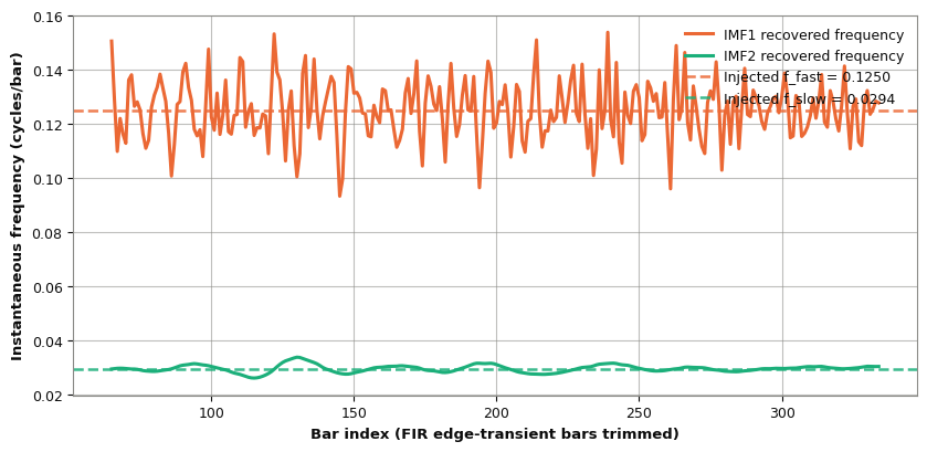
Fig. 3. Recovered instantaneous frequency for IMF1 and IMF2 (solid lines) against the known injected frequencies (dashed lines) after the FIR edge-transient bars are trimmed. IMF2 tracks its target almost exactly bar to bar; IMF1 shows more bar-to-bar scatter around the dashed line, consistent with its shorter cycle length, though its median still lands on the injected value.

Feeding that same synthetic signal through the full pipeline into the H(t,ω) matrix produces exactly the picture you would hope for: two clean, stable horizontal energy bands, one at each injected frequency, with no spurious energy smeared across the rest of the frequency axis.

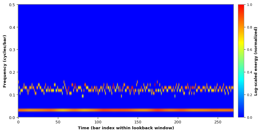
Fig. 4. The rendered H(t,ω) heatmap for the synthetic validation signal - the same visual the CCanvas panel produces live on chart. Two stable energy bands mark the two injected cycles.

A complementary diagnostic is the marginal Hilbert spectrum - energy integrated across the full time window for each frequency bin, collapsing the 2D surface into a 1D profile. It is a useful secondary readout when you want a single-glance summary of which cycle lengths have dominated over the current lookback window rather than watching the full live heatmap:

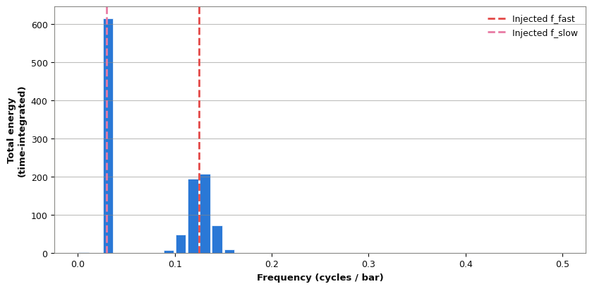
Fig. 5. Marginal spectrum: total energy per frequency bin over the validation window, peaking exactly at the two injected frequencies.

Being upfront about the limits of this kind of test: a synthetic two-sine-wave signal with known frequencies is a controlled check that the math chain is wired correctly end to end, not a guarantee about how cleanly EMD will separate cycles on real, noisy XAUUSD price action, where the number of dominant cycles isn't known in advance and can change mid-window. It should also be said plainly that verify_consistency.py is a deliberate line-by-line port of the MQL5 logic rather than an independent reference implementation, so agreement between the two confirms the MQL5 code matches its own Python mirror, not that either one has been checked against some outside ground truth.

That is why a second check matters as a separate step: watching the live panel redraw against real ticks in the Strategy Tester. The synthetic test validates the numerics; the live run confirms the indicator behaves correctly under the throttling, redraw, and array-orientation conditions it will actually run under. The Limitations section below goes further into what neither check actually proves.

For the second check - live rendering under real market data - run the indicator in the Strategy Tester's visual mode on XAUUSD, M5 (or your own symbol and timeframe) and step through ticks watching for three things: the canvas redraws cleanly on each new bar close, the bar-close throttle actually suppresses redundant recomputation between bar closes, and redraw latency stays visibly well under one bar's worth of time even with the full 200-bar lookback and six-IMF cap - if it doesn't, shorten the lookback or the IMF cap before trusting the panel on a fast timeframe.

This is a qualitative visual/performance check rather than a profit-and-loss backtest, since there is no order logic to evaluate, and it isn't a substitute for instrumenting the code yourself if you need a hard latency number (see Limitations, below). The reference parameters for that kind of run:

Setting	Value
Symbol / Timeframe	XAUUSD / M5
Applied price	Close
Rolling lookback	200 bars
Max IMFs	6
Frequency bins	40
Recalculation mode	Bar close only (throttled)

Note that any on-chart screenshots from this live run are visual/qualitative checks of the rendering pipeline, not performance backtests, and should be replaced with fresh Strategy Tester captures on your own broker feed before relying on the visual behavior for a specific symbol or session.

Limitations and What This Doesn't Prove

Every check above establishes something narrower than "this indicator works." Before you rely on the panel for anything beyond visual exploration, here is exactly what has and has not been verified.

The Python validation is not an independent ground truth. verify_consistency.py is a deliberate line-by-line mirror of the MQL5 sifting loop, FIR kernel, and phase-unwrap chain, built that way specifically so a mismatch between the two implementations shows up as a numerical discrepancy. Agreement between them confirms the MQL5 code does what its own Python port does, and both trace back to the same textbook EMD/Hilbert-transform formulas; it is not a check against an unrelated reference implementation, and it cannot catch a mistake both sides happen to share.

The synthetic test signal is intentionally simple. Two known sine waves plus a slow drift and Gaussian noise are enough to confirm the sifting-and-FIR chain recovers frequencies it should recover, but the signal has no gaps, volume spikes, sudden volatility clusters, or the sharp, asymmetric moves that tend to trigger EMD's mode-mixing failure mode. A pipeline that passes this test can still separate cycles less cleanly on a real, choppy XAUUSD session.

There is no quantitative real-data benchmark in this article. The XAUUSD M5 run described in the Testing section is a visual/qualitative check that the panel redraws correctly under live tick-driven bar updates, not a measurement of decomposition accuracy against real price - there is no known "correct" frequency decomposition of real market data to measure against, which is exactly why the synthetic test above exists as a separate, controlled check instead.

Redraw latency has not been benchmarked with instrumentation. "Redraw latency stays visibly well under one bar's worth of time" in the Testing section is guidance on what to watch for, not a measured figure from a profiler. If you need a hard number for your own broker feed and hardware, wrap the OnCalculate() body in GetMicrosecondCount() calls and log it yourself - the actual figure will vary with lookback, IMF cap, and machine.

Naive 3-point extrema detection is sensitive to noise and plateaus. FindExtrema() flags a point as an extremum only if it is strictly greater (or less) than both neighbors, so a flat plateau of equal values, or single-tick noise sitting on top of a real turning point, can add or drop an extremum that the underlying price structure didn't really have. That feeds straight into sifting quality, since the envelope is only ever as good as the extrema it is built from.

Frequency clipping to [0, 0.5] discards a diagnostic signal. A reading that gets floored or capped is exactly the kind of case worth surfacing separately - as noted earlier, a mode that clips repeatedly is often telling you it is poorly separated (mode mixing) rather than simply producing numerical noise, and the current implementation clips it away silently rather than logging or flagging the occurrence.

Frequency-bin resolution is coarse and linear. Forty bins spread evenly across [0, 0.5] cycles/bar give roughly 0.0125 cycles/bar per bin - fine enough to separate an 8-bar and a 34-bar cycle cleanly, as the validation figures show, but at the low-frequency end that same bin width covers a much wider range of actual periods than it does at the high-frequency end, so two genuinely different slow cycles can land in the same bin when two fast ones would not.

Historical heatmap columns can change as the window slides. Because EMD recomputes from scratch over the whole rolling window on every redraw rather than extending prior results incrementally, a column you saw earlier can take on a slightly different value once new bars enter the window and the sift re-partitions that stretch of price differently. This is a legitimate property of how sliding-window EMD works, not a bug, but it does mean the historical part of the panel is not frozen once drawn - treat it as a live analytical surface, not an immutable log.

Residual handling is a design choice, not a fixed rule. When sifting stops - either the SD criterion or a degenerate extrema count - whatever is left is folded into the residual rather than forced into one more IMF. That residual absorbs the slow trend by construction and is not itself analyzed for cycle content anywhere in this pipeline, so a genuinely slow oscillation that never separates cleanly from the trend simply will not appear on the heatmap.

Spline endpoints distort independently of the FIR edge transients. SplineEnvelope() holds the envelope flat before the first extremum and after the last one rather than extrapolating a curve, which is a separate source of edge distortion from the FIR kernel's zero-padding - it affects the envelope construction inside every sifting pass, not just the instantaneous-frequency readings at the very edges of the final window. The two effects compound near the boundaries of a short lookback rather than being interchangeable, so trimming only the FIR-transient bars does not fully clear spline-related edge artifacts from the earliest IMFs.

"Dominant" means highest-energy in the current window and binning, not a claim about a persistent market cycle. When this article or the panel itself calls a band "dominant," that is shorthand for "the highest-energy band in the current rolling window at the current frequency resolution" - it is not a claim that timeframe is objectively or persistently the market's real cycle. A different lookback length or a different moment in the slide can legitimately show a different band as dominant; treat it as a read on the current window, not a discovered constant.

None of this is a reason to avoid the indicator - it is the honest scope of what has actually been checked, so you can decide for yourself how much weight to put on any single reading before you build a strategy around it.

Conclusion

The Hilbert Spectrum turns "what cycle is the market in right now" from a vague, indicator-hopping question into a live, quantitative surface you can watch update bar by bar. EMD does the hard work of finding oscillatory modes without assuming a fixed basis, the FIR Hilbert transform turns each mode into instantaneous frequency and energy, and a straightforward binning-and-color-mapping step turns that into a heatmap your eyes can read at a glance. None of this predicts direction on its own - it is a lens, not a signal - but pairing it with your own entry logic gives you a genuinely different piece of information than moving averages or oscillators can offer: which timescale is actually dominating price action at this moment.

If you are picking parameters for your own symbol and timeframe rather than copying the XAUUSD M5 defaults, start with the lookback window: it should comfortably span several cycles of the slowest oscillation you actually care about, since EMD needs enough repetitions of a cycle in the window to separate it cleanly from the residual trend. From there, the FIR tap count and SD threshold are secondary tuning knobs - the defaults here are a reasonable starting point for most intraday forex and metals charts, but a much lower or higher timeframe may reward shortening or lengthening the kernel as discussed earlier.

A few natural directions to take this further: Ensemble EMD to reduce mode mixing at the cost of more CPU, adaptive frequency-bin resolution that widens at low frequencies and narrows at high frequencies, and cross-referencing the dominant IMF's instantaneous frequency against known session/news timing to see whether cycle-length shifts cluster around specific market events. All of the code here mirrors its Python validation counterpart exactly, so if you extend the MQL5 side, extend the Python side with it - that consistency is what let us catch problems numerically before ever loading the indicator on a live chart.

File	Type	Description
HilbertSpectrum.mq5	Indicator	Main custom indicator: OnInit feature-contract checks, BuildSource price extraction, bar-close-throttled OnCalculate, live canvas draw.
EMD.mqh	Include	CEMD class: sifting algorithm (SiftOnce), full decomposition loop (Decompose), cubic-spline envelopes, Cauchy SD stopping criterion.
HilbertTransform.mqh	Include	CHilbertTransform class: FIR Hilbert kernel, quadrature convolution, instantaneous amplitude/phase/frequency.
SpectrumCanvas.mqh	Include	CCanvas-based heatmap renderer with log-scaled energy colormap.
verify_consistency.py	Python	Offline mirror of the EMD + FIR Hilbert pipeline for numerical validation against known-frequency synthetic signals. Ships in the archive under MQL5\Files\HilbertSpectrum\Python\.
MQL5.zip	Archive	Full package rooted at MQL5\, ready to extract straight into your MQL5 data folder: Include\HilbertSpectrum\, Indicators\HilbertSpectrum\, and Files\HilbertSpectrum\Python\ for the validation script above. No compiled .ex5 binaries are included - compile the .mq5 sources yourself in MetaEditor before running the indicator.