Neural Networks in Trading: Adaptive Perception of Market Dynamics (STE-FlowNet)

Introduction

In recent years, financial markets have been undergoing a rapid transformation driven by deep learning. The challenge of creating models capable not only of identifying patterns in data but also of forming a robust representation of the temporal, contextual, and structural aspects of market dynamics is becoming increasingly pressing. Against this backdrop, the STE-FlowNet framework stands out; proposed in the article "Spatio-Temporal Recurrent Networks for Event-Based Optical Flow Estimation," it demonstrates a new approach to processing event sequences. In this system, each step does not merely reflect current data, but dynamically reconfigures the system's internal representation, adapting to changes in the information flow being analyzed.

The financial market is an extremely complex and nonlinear system, prone to sudden market regime disruptions, cascading reactions, and rare but significant patterns. Classical recurrent models, such as LSTM and GRU, often exhibit inertia under these conditions. They either average over the history, overlooking important short-term events, or overreact to noise. The STE-FlowNet framework takes a different approach to solving this problem. It dynamically adjusts its internal representations by adapting filters and temporal sensitivity to specific market scenarios. This behavior is reminiscent of an experienced trader who interprets events in the context of changing conditions.

A key advantage of STE-FlowNet is its ability to handle the evolution of market states. The framework tracks the dynamics of hidden structures, which is particularly important when modeling regime shifts, liquidity spikes, and changes in the balance of power among participants. Instead of making point predictions about the continuation of a time series, the model learns to perceive the course of events by adapting its internal representations to new conditions. This approach transforms forecasting into adaptive perception, which is particularly valuable for developing robust trading strategies.

The architectural philosophy focuses on dynamic market perception. The past is viewed as a flexible map of trajectories that adapts to new events. This allows the model to remain relevant over long-term dependencies while also capturing critical short-term events. The proposed data processing method is particularly valuable for financial markets, where it is important not only to record historical data but also to interpret shifts in its structure.

Today, as market patterns become less predictable and periods of relative equilibrium are interrupted by sharp phase shifts, adaptive models have become a necessity. Traditional analytical methods often fail: they either capture outdated features or react too late, when the market structure has already changed. This is precisely where the framework under consideration demonstrates its advantage, enabling it to adapt to the new rules of the game almost instantly.

The model conceptualizes the market as a dynamic system. Each new signal updates the state and reinterprets the context of previous observations. This brings the algorithm closer to the thinking of a professional trader who actively refines hypotheses about the current market regime. The result is a tool capable of recognizing changes in context in a timely manner and adapting its strategy — which is critically important for financial applications.

The framework's architecture is designed from the outset for practical adaptability: it assesses the current market phase and adjusts its internal logic of perception in real time, ensuring model robustness when the market regime changes. This makes it particularly valuable for developing strategies that can respond to changes in context, not just to price motion.

The STE-FlowNet Algorithm

The STE-FlowNet framework is built around the concept of spatiotemporal recurrent event processing, which enables the analysis of complex data sequences with a high degree of accuracy. The model receives a stream of events from the cameras and gradually builds an internal representation of motion, taking each new event into account and constantly updating its internal memory.

Each block of the model processes short sequences of events, carefully analyzing them in terms of their spatial and temporal dependencies. This makes it possible to detect motion even at high speeds and in dynamically complex scenes, where traditional methods often miss important details.

A stable representation of the dynamics is gradually formed, making it possible to predict future developments with a high degree of accuracy. The network's internal state contains local and global characteristics of motion, which enables the model to capture complex structures and predict patterns across various time scales.

The representation of the input data in STE-FlowNet is based on the operating principles of event cameras, which respond to changes in the logarithm of brightness intensity that exceed a specified threshold θ. Each event records the pixel coordinates, timestamp, and polarity of the change (increase or decrease in brightness), which can be written as e = {x, t, p}. In the context of financial markets, an analogy can be drawn to the execution of a trade, which results in a change in price or volume. Each entry contains critically important information about the system's current state and can serve as a signal for analyzing market dynamics. This makes the event stream a rich source of data capable of identifying even subtle trends and sharp fluctuations.

The event stream, however, may be partially lost due to pixel bandwidth limitations, especially in high-speed, complex-textured scenes. In a financial context, this is similar to missing individual trades or momentary price fluctuations in active markets. Traditional methods of summarizing or aggregating data often fail to capture rapid changes and overlook short-term patterns. To address this issue, the framework’s authors proposed a modified representation of the data being analyzed that amplifies the signal and makes it possible to identify critical events that shape the system’s subsequent dynamics.

All events are divided into N equal parts by count. Simply summing events to form an image does not reflect the actual details of motion over the period. If events are concentrated within a short time interval, this indicates high activity, whether it involves the rapid motion of objects in a scene or a surge in trading activity in the market. To account for these characteristics, a weighting scale based on the temporal distribution of events is introduced. High-density events are assigned greater weight, allowing STE-FlowNet to focus on significant moments and ignore less critical fluctuations.

For a set of M events (xi, yi, ti, pi), where i ∈ [1:M], a Gaussian model is applied in a single block to approximate their temporal distribution. Each event is assigned a corresponding weight.

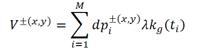
Here, kg(a) is the sampling kernel based on the Gaussian model, µ is the mean value of the timestamps, σ is the variance calculated over all M events, and λ is the normalization coefficient.

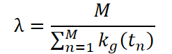
The more concentrated the distribution of events is over time, the greater their weight. This allows the model to identify periods of intense activity. In a financial context, this makes it possible to identify periods of heightened volatility, sharp spikes in trading volume, or anomalies that may signal key market turning points. All weighted values are rounded up to preserve the significance of each event and avoid losing critical information about rapid changes.

Thus, the STE-FlowNet model becomes capable of detecting micro-movements and patterns that are typically lost during standard data aggregation, and of using them to generate more accurate forecasts, assess risks, and develop highly adaptive strategies.

The overall architecture of STE-FlowNet is a variant of an Encoder-Decoder model. Each event-image passes through four encoder modules, each of which doubles the number of output channels and halves the data resolution. After that, the feature maps obtained from the encoders pass through two residual blocks, which enhances the feature representation and maintains gradient stability.

In addition, there is a skip connection between each encoder level and the corresponding decoder, which ensures a direct flow of information while preserving important local and global features. As the data passes through the decoder stage, it undergoes a transposed convolution to double the resolution. After passing through all four decoder modules, the image is restored to its original size. This structure allows the model to accurately reproduce spatial details and preserve the critical characteristics of event dynamics.

STE-FlowNet also generates intermediate flow maps (intermediate flow) at each resolution, which are then used as part of the input data for the next decoder. During training, the loss function is applied to all intermediate maps, which improves training and increases prediction accuracy. This architecture is particularly useful for financial flows, where it is important to track both short-term and long-term patterns simultaneously: intermediate flows help capture micro-price movements, sharp spikes in volume, and other significant events, creating a more reliable and adaptive analytical model.

A key component of feature extraction in STE-FlowNet is ConvGRU, which plays a central role in processing spatiotemporal information. Although ConvGRU has already been used in some studies involving frame-based data, its functionality was previously limited to the use of high-level feature maps from the upper layers of a ConvNet. However, most of the local information is lost, and temporal variations between frames are often smoothed out. This makes it difficult to accurately detect subtle motions and rapid changes.

In the context of financial flows, this is comparable to the loss of information about short-term price fluctuations or small-scale transactions, which can be critical for making trading decisions and assessing market risks. To address this issue, the authors of the STE-FlowNet framework proposed encoder modules that use ConvGRU to sequentially extract spatiotemporal features at different resolution levels, while preserving local motion patterns and dynamic details. This makes it possible to track even the slightest changes in the data flow.

The event-image being analyzed passes through two parallel architectures resembling a pyramid. The first path is through a ConvNet, which generates spatial feature maps at different resolution levels, providing global context and capturing the overall structure of the event. The second path passes through spatiotemporal encoders at each level. Each encoder includes a ConvGRU and a strided convolution. This approach provides the model with information about rapid local fluctuations as well as slower global trends. In financial analysis, this can be interpreted as simultaneously tracking short-term spikes in trading activity and long-term market trends, which improves the accuracy of forecasts and allows for the identification of critical points for strategic decisions.

At each time step t, the ConvGRU input consists of three key components:

• feature maps Fst,t from the underlying spatio-temporal encoder,
• the hidden state ht-1 from the previous step,
• the output of the correlation layer Ct at the same resolution level.

ConvGRU is defined by the following equations:

The correlation layer calculates the correspondence between the spatial feature maps of the current event Fst,t and the first event Fs,1, using the predicted flow f* from the previous iteration.

The step-by-step construction of the flow prediction, based on information from previous steps, is similar to the analytical work of a trader who evaluates each new trade in the context of previous events. This makes it possible to model the evolution of market processes more accurately, identify potential entry and exit points, and develop adaptive strategies capable of responding quickly to changes in the market environment.

In addition, this architecture improves the model’s robustness to noise fluctuations, anomalies, and rare events, creating a reliable tool for comprehensive analysis of financial flows and decision support in highly competitive markets.

To improve the accuracy and reliability of forecasts, STE-FlowNet uses an iterative refinement scheme. Each iteration generates a residual flow ∆fk, which is accumulated with the previous estimate fk-1 to form an updated prediction fk = fk-1 + ∆fk, starting from f0 = 0.

Reusing the same block with shared weights ensures consistency across iterations, conserves resources, and promotes training stability. Intermediate predictions serve two purposes. First, they are used as part of the input data for the next iteration, ensuring accurate corrections based on previous estimates. Second, they act as a skip connection that adds the predicted flow to the model's current output, allowing the prediction to be refined with a high level of detail. This multi-stage strategy is similar to a step-by-step analysis of financial forecasts, in which each new estimate of price, volume, or an indicator is refined based on all previous data, creating an adaptive and accurate model of market movement.

The iterative process allows not only the sequence of events to be taken into account, but also potential noise, rare events, and sharp fluctuations, thereby increasing the model's robustness to financial market instability. This enables the generation of highly detailed and reliable forecasts. STE-FlowNet is capable of processing large volumes of events, capturing every significant motion, integrating it into the overall picture, and providing a comprehensive view of the current state of the market.

The recurrent and iterative architecture of STE-FlowNet allows events to be processed frame by frame, taking into account the entire sequence of preceding changes. In a financial application, this means the ability to accurately capture instantaneous price fluctuations and sharp spikes in trading activity, as well as to identify rare and anomalous events, while taking global market trends into account. Iterative refinement ensures that the model dynamically adapts to new data, enabling the generation of highly reliable, detailed, and predictable forecasts — which is critically important for comprehensive risk analysis, adaptive capital management, and strategic planning in rapidly changing and volatile markets, where every millisecond can significantly impact the outcome of decision-making.

To train STE-FlowNet, the framework's authors use synchronized streams of events and grayscale images, which enables self-supervised learning. The stream of events between two consecutive images (It, It+dt) is converted into a sequence of event-images, which are fed into the network one after another. At the same time, the predicted flow f = (f¹, f²) is applied to the second image to generate the warping, which makes it possible to compute the error and train the model without explicit annotations. This approach enables STE-FlowNet to learn to accurately estimate the motion of events even in conditions with complex dynamics.

The loss function includes two key components: photometric reconstruction Lphoto and flow smoothness Lsmooth, and is expressed as:

where λ controls the weight given to smoothness relative to photometric accuracy. Photometric loss quantifies the discrepancy between the first image and the transformed second image, taking into account the predicted flow:

where ρ is the Charbonnier Loss, ρ(x) = (x² + η²)^r with r = 0.45 and η = 1e-3. The more precise the flow, the smaller the discrepancy, which allows the model to capture the slightest changes and details that are critical for analyzing rapid events.

Flow smoothness Lsmooth minimizes the differences between neighboring pixels, enhancing the spatial consistency of the flow and reducing local errors. In a financial context, this is analogous to smoothing out random noise and spikes in trading volume while preserving significant short-term changes in prices and activity. This mechanism allows the model to simultaneously track local anomalies — sudden changes in quotes and spikes in trading activity — and global trends.

The use of photometric and smoothness losses creates a balanced training strategy. The model captures instantaneous movements and trends while avoiding overfitting to noisy or rare events. In financial flows, this enables the creation of forecasts that can respond accurately to market fluctuations, identify anomalies, and provide real-time decision support, ensuring the reliability and adaptability of trading strategies in dynamic markets. Thanks to this integration of spatiotemporal analysis and self-supervised learning, STE-FlowNet becomes a tool capable of identifying patterns at the microsecond level while also accounting for long-term trends, making it valuable for strategic planning and risk management.

The author's visualization of the STE-FlowNet framework is shown below.

Implementation in MQL5

After a detailed examination of the theoretical aspects of the STE-FlowNet framework, we move on to the practical part of our work, where we will focus on one possible implementation of the proposed approaches using MQL5. It should be emphasized that our implementation is not an exact copy of the original version of the framework. We adapt the model's core ideas and key principles to work with market data. In particular, we transfer the concept of spatiotemporal processing and iterative flow refinement into the framework for analyzing prices, volumes, and other trading indicators.

This approach allows us to leverage the advantages of STE-FlowNet in the context of financial market analysis: to capture short-term spikes in trading activity, abnormal price fluctuations, and sharp changes in volume, while simultaneously taking long-term trends into account. Implementation using MQL5 makes it possible to integrate the model directly into trading strategies and algorithmic systems, enabling both offline testing on historical data and adaptive real-time forecasting. In addition, using MQL5 makes it possible to optimize computational processes, ensuring efficient processing of large streams of market data and the sequential application of spatiotemporal filters, which is critical for high-frequency trading and risk analysis.

Thus, our practical work not only applies the STE-FlowNet architecture to financial data but also extends its functionality, creating a flexible tool for analyzing market dynamics, forecasting short-term and long-term changes, and developing reliable trading strategies that take real market conditions into account.

However, it should be noted that the architecture of the STE-FlowNet framework is quite complex. The authors use a variety of modules distributed across several information streams, which allows the model to process data at different levels of abstraction and account for both local and global changes. Naturally, we will take a gradual, step-by-step approach to fully implementing this architecture, adapting its key elements to the analysis of financial data. This phased approach will allow us to study the characteristics of individual components, adjust the algorithms to market specifics, and ensure the model’s stability when integrated into trading strategies.

We will begin our work by building one of the framework's core modules — ConvGRU. For simplicity, we assume that an already concatenated tensor of features and correlations is fed into the module. This will allow us to focus on extracting spatiotemporal dependencies and processing information about the dynamics of market events before integrating more complex multi-stream structures. In addition, this approach allows us to build a more versatile object that is not tied to a specific architectural solution.

The module's algorithm is implemented in a new class, CNeuronSpikeConvGR, which inherits base functionality from the CNeuronSpikeActivation object. This parent-class object indicates the spiking nature of the object being created.

class CNeuronSpikeConvGRU  :  public CNeuronSpikeActivation
  {
protected:
   CNeuronBaseOCL       cConcatenated[2];
   CNeuronConvOCL       cZR;
   CNeuronBaseOCL       cZ;
   CNeuronBaseOCL       cR;
   CNeuronConvOCL       cHt;
   CNeuronBaseOCL       cH;
   CNeuronBatchNormOCL  cNorm;
   //---
   virtual bool      feedForward(CNeuronBaseOCL *NeuronOCL) override;
   virtual bool      updateInputWeights(CNeuronBaseOCL *NeuronOCL) override;
   virtual bool      calcInputGradients(CNeuronBaseOCL *NeuronOCL) override;
   
public:
                     CNeuronSpikeConvGRU(void) {};
                    ~CNeuronSpikeConvGRU(void) {};
   //---
   virtual bool      Init(uint numOutputs, uint myIndex, COpenCLMy *open_cl,
                          uint units, uint chanels_in, uint chanels_out,
                          ENUM_OPTIMIZATION optimization_type, uint batch);
   //---
   virtual int       Type(void)   override const   {  return defNeuronSTFS;   }
   //--- methods for working with files
   virtual bool      Save(int const file_handle) override;
   virtual bool      Load(int const file_handle) override;
   //---
   virtual void      SetOpenCL(COpenCLMy *obj) override;
   virtual void      SetActivationFunction(ENUM_ACTIVATION value) override;
   //---
   virtual bool      WeightsUpdate(CNeuronBaseOCL *source, float tau) override;
  };

In the structure of the new class presented here, we see a number of internal objects:

• cConcatenated — stores a concatenated tensor of the analyzed data, including feature maps, correlation maps, and the hidden state;
• cZR — a convolution module responsible for computing the Z (update) and R (reset) gates that control the state of the hidden layer;
• cZ and cR — separate structures for storing the values of the update and reset gates at the current step;
• cHt — stores an intermediate hidden state after applying gates and convolutions;
• cH — the hidden state of a neuron, which is updated at each step and used in subsequent iterations;
• cNorm — a batch normalization module designed to stabilize and accelerate training; it prepares the data before spiking activation is performed by the parent class.

All of the object's internal components are declared statically, which allows the class's constructor and destructor to be left empty. The object is initialized in the Init method, which assembles all internal submodules into a working chain. This is important. After all, our ConvGRU is not a separate black box, but part of the overall spatiotemporal processing in STE-FlowNet. Accordingly, each step of the initialization process is designed with data flow and computational efficiency in mind.

bool CNeuronSpikeConvGRU::Init(uint numOutputs,uint myIndex,COpenCLMy *open_cl,
                               uint units,uint chanels_in,uint chanels_out,
                               ENUM_OPTIMIZATION optimization_type,uint batch)
  {
   if(!CNeuronSpikeActivation::Init(numOutputs,myIndex,open_cl,units*chanels_out,optimization_type,batch))
     return false;

The first line of code within the method performs the basic initialization of the parent class object. Here, we allocate memory, bind the object to an OpenCL context, and set the size of the result tensor.

Next comes the initialization of the internal components. The first one is cConcatenated. Its task is to combine the input data with the hidden state.

   uint index = 0;
   for(uint i = 0; i < cConcatenated.Size(); i++)
     {
      if(!cConcatenated[i].Init(0, index, OpenCL, units * (chanels_in + chanels_out), optimization, iBatch))
         return false;
      cConcatenated[i].SetActivationFunction(None);
      index++;
     }

For this object, we explicitly disable the activation function. And that makes sense. After all, what we have here is simply a buffer that combines the tensors of two information streams, which may have undergone different nonlinear transformations.

The next cZR is a convolution module for computing Z and R.

   if(!cZR.Init(0,index,OpenCL,chanels_in+chanels_out,chanels_in+chanels_out,
				2*chanels_out,units,1,optimization, iBatch))
      return false;
   cZR.SetActivationFunction(SIGMOID);

Here, we create a convolutional block that outputs values for two gates simultaneously: Z controls the memory update, and R controls the reset scale for the previous state. In other words, in a single pass, we get two sets of maps — one for each gate. The SIGMOID activation function is the standard for gates: its output lies in the range (0, 1).

To simplify the calculations, we split the combined gate tensor into two components.

   index++;
   if(!cZ.Init(0,index,OpenCL,cZR.Neurons()/2,optimization,iBatch))
      return false;
   cZ.SetActivationFunction((ENUM_ACTIVATION)cZR.Activation());
   index++;
   if(!cR.Init(0,index,OpenCL,cZR.Neurons()/2,optimization,iBatch))
      return false;
   cR.SetActivationFunction((ENUM_ACTIVATION)cZR.Activation());

From an architectural standpoint, this provides flexibility: in future versions, cZR can be replaced with a more complex module, while cZ and cR will remain interfaces.

Next, we initialize cHt — a module for computing the candidate hidden state.

   index++;
   if(!cHt.Init(0,index,OpenCL,chanels_in+chanels_out,chanels_in+chanels_out,
                                   chanels_out,units,1,optimization, iBatch))
      return false;
   cHt.SetActivationFunction(TANH);

Here, we use a separate convolutional block. The inputs are the same — a combination of features and the previous state (in our concatenated representation). The output is the feature dimension at the module output. TANH activation is the standard for a candidate hidden state: it centers the signal and produces a range of (−1, 1). In a trading context, this helps keep the response within reasonable limits and prevent value explosions.

And the hidden state itself, cH.

   index++;
   if(!cH.Init(0,index,OpenCL,Neurons(),optimization,iBatch))
      return false;

This object stores the final hidden state h. It is important to note that we separate the computational component cHt from the state storage cH. This design makes it easier to track state versions during iterative refinement.

The method concludes by initializing the batch normalization object cNorm.

   index++;
   if(!cNorm.Init(0,index,OpenCL,Neurons(),iBatch,optimization))
      return false;
      cNorm.SetActivationFunction(None);
//---
   return true;
  }

BatchNorm adjusts the distribution of pre-activation responses.

The feedForward method performs a complete forward pass through the ConvGRU module, sequentially updating the hidden state based on the current input and the stored memory.

bool CNeuronSpikeConvGRU::feedForward(CNeuronBaseOCL *NeuronOCL)
  {
   if(!NeuronOCL)
      return false;
//---
   uint units = cHt.GetUnits();
   uint hidden = cHt.GetFilters();
   uint inputs = cHt.GetWindow() - hidden;

First, we calculate the module's key parameters:

• units represents the spatial partitioning of the input,
• hidden specifies the number of output state channels,
• inputs is the number of input channels in the original feature tensor.

Next, the SwapOutputs method is called, preparing the cH buffer for updating by saving the previous state for computing the recurrent component.

   if(!cH.SwapOutputs())
      return false;

The input features being analyzed are then concatenated with the previous hidden state, forming the first input for computing the Z and R gates.

   if(!Concat(NeuronOCL.getOutput(), cH.getPrevOutput(), cConcatenated[0].getOutput(), inputs, hidden, units))
      return false;

The cZR block performs a convolutional forward pass, generating combined gate maps that are then split into cZ and cR.

   if(!cZR.FeedForward(cConcatenated[0].AsObject()))
      return false;
   if(!DeConcat(cZ.getOutput(), cR.getOutput(), cZR.getOutput(), hidden, hidden, units))
      return false;

After that, the R gate masks the previous state through element-wise multiplication, which implements a partial memory reset mechanism.

   if(!ElementMult(cR.getOutput(), cH.getPrevOutput(), cR.getPrevOutput()))
      return false;

The concatenation of the current inputs and the modified state is fed into the second convolutional block, cHt, which computes a candidate hidden state.

   if(!Concat(NeuronOCL.getOutput(), cR.getPrevOutput(), cConcatenated[1].getOutput(), inputs, hidden, units))
      return false;
   if(!cHt.FeedForward(cConcatenated[1].AsObject()))
      return false;

Next, the GateElementMult function combines the old and new states via the Z gate, smoothly controlling the degree of memory update.

   if(!GateElementMult(cHt.getOutput(), cH.getPrevOutput(), cZ.getOutput(), cH.getOutput()))
      return false;

The resulting output passes through the cNorm normalization layer, after which it is activated by the parent class, completing the forward-pass phase.

   if(!cNorm.FeedForward(cH.AsObject()))
      return false;
   if(!CNeuronSpikeActivation::feedForward(cNorm.AsObject()))
      return false;
//---
   return true;
  }

This step-by-step mechanism allows the module to strike a precise balance between maintaining long-term context and responding instantly to new market signals.

Thus, CNeuronSpikeConvGRU implements the full operational logic of the ConvGRU module, making it possible to gradually integrate it into market event analysis, capture short-term fluctuations, and learn from historical data to build adaptive trading strategies.

We've worked hard today, and it's time to take a short break. Let your thoughts settle calmly and fall into place, and in the next article we will return to development with renewed energy and continue moving forward.

Conclusion

In this article, we explored the STE-FlowNet framework, which offers a fundamentally different approach to processing dynamic data thanks to its event-based perception model. Its architecture demonstrates how spatiotemporal dependencies can be extracted not according to fixed time intervals, but according to actual changes in the signal structure. That is exactly what traditional approaches to financial markets so sorely lack. It is capable of capturing local and temporal dependencies without losing detail, preserving subtle changes in the flow structure where classical models simply average them out. This approach preserves the dynamics, is not tied to fixed timeframes, and lets the forecast be refined step by step, as if observing the evolution of market momentum in real time.

Links

• Spatio-Temporal Recurrent Networks for Event-Based Optical Flow Estimation
• Other articles in this series

Software used in this article

#	Name	Type	Description
1	Study.mq5	Expert Advisor	Expert Advisor for offline model training
2	StudyOnline.mq5	Expert Advisor	Expert Advisor for online model training
3	Test.mq5	Expert Advisor	Expert Advisor for model testing
4	Trajectory.mqh	Class library	Structure describing the system state and model architecture
5	NeuroNet.mqh	Class library	Class library for creating a neural network
6	NeuroNet.cl	Library	Code library for an OpenCL program