Comparing Trade Return Distributions with Mann-Whitney U in MQL5

Introduction

A common practice when evaluating a trading strategy across two market periods is to compute the average return in each period and compare the two numbers. This comparison is fast and intuitive, but it is statistically unreliable for trade return data. Trade returns are skewed by asymmetric win/loss structures, exhibit fat tails from slippage and gap events, and are frequently dominated by a handful of outlier trades that pull the mean away from where the bulk of the distribution sits. Two periods can have nearly identical mean returns while having distributions that look nothing alike.

MQL5 has no built-in non-parametric test for comparing two return samples without assuming a distribution shape. This article builds one. The implementation has three components:

• CMannWhitneyTest: pools both samples, assigns ranks, computes the U statistic with tie correction, and derives a z-score and p-value
• CBoxPlotRenderer: draws a dual box-and-whisker chart on a shared canvas so the two distributions are directly comparable by eye
• MannWhitneyDemo: extracts per-trade returns from closed trade history and connects the two components above

The full workflow is: ExtractReturns pulls two date-windowed return samples from the terminal's trade history, CMannWhitneyTest performs the statistical test, CBoxPlotRenderer plots the result, and the demo script connects all three. The complete source files are included in the archive attached at the end of the article.

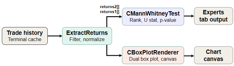
Architectural diagram showing how MannWhitneyDemo wires trade history through ExtractReturns into CMannWhitneyTest (statistical output) and CBoxPlotRenderer (visual output).

Section 1: Why Mean Comparisons Fail for Trade Returns

The t-test for two independent samples assumes the sampling distribution of the mean is approximately normal. Trade return distributions violate this assumption even at moderate sample sizes, because the distortions that matter — skew and tail weight — do not wash out quickly with more observations.

Consider two 30-day evaluation periods with 40 trades each. Period A's returns cluster tightly (+0.3% to +0.8%, a few -0.5% losses). The mean is approximately +0.31% and the median is +0.45%. Period B wins more often but two trades return -4.5% and -5.0% from adverse gap events. Those two outliers drag the mean to approximately +0.02%, even though the median is +0.15% and most Period B trades outrank most Period A trades on a pairwise basis. A t-test, inflated by the outliers' effect on variance, often fails to reject equal means at the 0.05 level despite the distributional difference being real.

The Mann-Whitney test ranks every return by its position in the pooled sample rather than by its magnitude. The two -4.5% and -5.0% losses in Period B occupy the bottom two ranks regardless of whether they are -1% or -50%. They cannot single-handedly dominate the test statistic the way they dominate the mean. The test correctly identifies that Period A's distribution is stochastically larger.

This distinction matters because Mann-Whitney does not test equality of means. It tests whether two populations share the same distribution, against the alternative that one is stochastically larger — that a randomly drawn observation from one group tends to rank above one from the other. For a trader deciding whether two market regimes warrant different parameter sets, this is the more relevant question.

The table below summarizes the key differences:

Criterion	t-test	Mann-Whitney U
Null hypothesis	Equal population means	Identical distributions
Distribution assumption	Approximately normal	None
Effect of one extreme trade	Can shift the mean and inflate variance	Bounded to one rank position
What it detects	Shift in average value	Any difference in location, spread, or shape
Output	p-value on mean difference	p-value on stochastic dominance

Two example return distributions with the same number of trades. Period A's mean and median nearly coincide; Period B's mean is pulled left by two outlier losses while its median remains representative of the typical trade.

Section 2: The Mathematics of the Mann-Whitney U Test

Ranking: Pool all n₁ + n₂ observations and rank them from 1 to n₁ + n₂ in ascending order, keeping each observation's group label. When k observations share an identical value, each receives the average of the ranks their block would have occupied. For example, three tied values at positions 3, 4, 5 each receive rank (3+4+5)/3 = 4.

The U statistic: Sum the ranks per group to get R₁ and R₂, then compute:

U₁ = R₁ − n₁(n₁ + 1) / 2
U₂ = R₂ − n₂(n₂ + 1) / 2

U₁ + U₂ = n₁·n₂ always holds and serves as a verification check. The test statistic is U = min(U₁, U₂). Taking the minimum rather than one specific Uᵢ makes the test two-sided: extreme values of either U₁ or U₂ indicate stochastic dominance in either direction, and min(U₁, U₂) captures whichever tail is more extreme.

Normal approximation: For sample sizes that are not very small, U under H₀ is approximately normal with:

μ_U = n₁·n₂ / 2
σ²_U = n₁·n₂·(n₁ + n₂ + 1) / 12

Ties reduce the discriminating power of the rank sums, so the variance requires a downward correction:

σ²_U (corrected) = n₁·n₂/12 · [(n₁+n₂+1) − Σ(t³−t) / ((n₁+n₂)(n₁+n₂−1))]

where the sum runs over every tied group of size t. Untied observations contribute zero since t³−t = 0 when t = 1. From the corrected variance:

z = (U − μ_U) / σ_U
p = 2 · (1 − Φ(|z|))

A two-tailed test is used throughout because the article makes no prior assumption about which period should rank higher. If the trader has a strong directional hypothesis going in, the one-tailed p-value is simply 1 − Φ(|z|) rather than the doubled value, and the sign of z from GetZ() identifies which group is ranked higher.

MQL5 has no built-in Φ, so the implementation uses the Zelen and Severo rational polynomial approximation from Abramowitz and Stegun, formula 26.2.17, with a maximum absolute error of approximately 7.5×10⁻⁸:

Φ(z) ≈ 1 − φ(z)·(b₁t + b₂t² + b₃t³ + b₄t⁴ + b₅t⁵),   t = 1/(1 + 0.2316419·z)

for z ≥ 0, using Φ(−z) = 1 − Φ(z) for negative z. This approximation is accurate enough for hypothesis testing at any conventional significance level. An exact permutation-based p-value would be more reliable below 20 observations per group, but the normal approximation is sufficient and far simpler to implement natively.

The exact permutation distribution of U requires enumerating all possible rank assignments across both groups, which grows exponentially with sample size and is computationally impractical for the trade-count ranges this implementation targets. The normal approximation becomes reliable above roughly 20 observations per group, which is the minimum the demo script recommends before trusting the result.

Some textbook presentations of the Mann-Whitney test apply a continuity correction of 0.5 to the numerator of the z-score, adjusting for the fact that a continuous distribution is being used to approximate a discrete one. This implementation omits it. At sample sizes where the normal approximation is already reliable — above 20 observations per group — the correction has a negligible effect on the p-value and adds no practical benefit. Below that threshold the approximation itself is the dominant source of error, not the discreteness adjustment, so the correction would give a false impression of precision on data that does not support it.

Box plot quartiles: Each group is summarized with the five-number summary using Tukey's hinges: Q2 is the median of the full sorted sample; Q1 is the median of the lower half; Q3 is the median of the upper half. When the sample size is odd, the median itself is excluded from both halves. Quartile computation sits in CMannWhitneyTest rather than in the renderer because it is a statistical operation, not a drawing operation, and keeping it in the statistics class allows it to be tested independently.

Section 3: Reading Trade History in MQL5

The demo extracts per-trade returns from two user-defined date windows using HistorySelect(), which loads deals into a cache, HistoryDealsTotal(), and HistoryDealGetDouble() and HistoryDealGetInteger() for individual deal properties.

A MetaTrader 5 position is composed of at least two deals: one that opens it and one that closes it. Only the closing deal carries the realized profit for that round trip. DEAL_ENTRY_OUT identifies closing deals. Opening deals are excluded because including them would double the sample size with zero-outcome entries, corrupting both the rank computation and the box plot.

The return for each qualifying trade is computed as:

normalized_return = profit / (volume * tick_value)

This is not a classic percentage return on capital or on the entry price. It is a normalized monetary return that makes trades of different volumes comparable on a consistent scale. A trade earning $50 with a volume of 1.0 lot on a pair with a tick value of $10 produces a different raw profit than the same directional move traded at 0.5 lots, but their normalized returns will differ proportionally. This is the correct basis for comparing trades across windows that may have used different position sizes.

The code retrieves SYMBOL_POINT and checks it is positive before proceeding, as a general validity guard on the symbol data, but the point itself does not appear in the return formula. If a point is zero or unavailable, it is a signal that the symbol's market data is unreliable for that deal, and the deal is skipped.

Three exclusions apply. Zero-volume deals are excluded because dividing by zero volume is invalid; these typically represent balance or credit adjustments. Deals on a different symbol than the one being analyzed are excluded because pooling returns across instruments with different volatility scales would make the rank comparison meaningless. Zero-profit deals with valid volume are kept, since a breakeven exit is a legitimate trade outcome.

Section 4: Implementation — MannWhitneyTest.mqh

CMannWhitneyTest takes two numeric arrays and produces the U statistic, z-score, and p-value. It has no knowledge of trade history, chart objects, or input parameters — just two arrays in, a test result out. This makes it independently testable and reusable in any context where two numeric samples need a distribution-free comparison.

The class declaration and key members:

//+------------------------------------------------------------------+
//|                                              MannWhitneyTest.mqh |
//+------------------------------------------------------------------+
#ifndef MANNWHITNEYTEST_MQH
#define MANNWHITNEYTEST_MQH

//+------------------------------------------------------------------+
//| Helper structure used while ranking the pooled sample            |
//+------------------------------------------------------------------+
struct SRankItem
  {
   double            value;
   int               index;
   double            rank;
  };

//+------------------------------------------------------------------+
//| Class CMannWhitneyTest                                           |
//| Purpose: implements the Mann-Whitney U test for two independent  |
//| samples, using the normal approximation with tie correction.     |
//+------------------------------------------------------------------+
class CMannWhitneyTest
  {
private:
   double            m_group1[];
   double            m_group2[];
   int               m_n1;
   int               m_n2;
   double            m_U1;
   double            m_U2;
   double            m_U;
   double            m_z_score;
   double            m_p_value;
   double            m_tie_sum;

   void              RankPooled(double &ranks[]);
   double            NormalCDF(double z);
   void              SortRankItems(SRankItem &items[]);

public:
                     CMannWhitneyTest(void);
                    ~CMannWhitneyTest(void);

   void              SetGroup1(const double &data[]);
   void              SetGroup2(const double &data[]);
   bool              Run(void);
   double            GetU(void) const;
   double            GetZ(void) const;
   double            GetP(void) const;
   void              PrintResult(double alpha);
   void              ComputeQuartiles(const double &data[],double &q1,double &q2,double &q3);
  };

//+------------------------------------------------------------------+
//| Constructor                                                      |
//+------------------------------------------------------------------+
CMannWhitneyTest::CMannWhitneyTest(void)
  {
   m_n1=0;
   m_n2=0;
   m_U1=0.0;
   m_U2=0.0;
   m_U=0.0;
   m_z_score=0.0;
   m_p_value=1.0;
   m_tie_sum=0.0;
  }

//+------------------------------------------------------------------+
//| Destructor                                                       |
//+------------------------------------------------------------------+
CMannWhitneyTest::~CMannWhitneyTest(void)
  {
  }

//+------------------------------------------------------------------+
//| Copy the first sample into internal storage                      |
//+------------------------------------------------------------------+
void CMannWhitneyTest::SetGroup1(const double &data[])
  {
   m_n1=::ArraySize(data);
   ::ArrayResize(m_group1,m_n1);
   ::ArrayCopy(m_group1,data);
  }

//+------------------------------------------------------------------+
//| Copy the second sample into internal storage                     |
//+------------------------------------------------------------------+
void CMannWhitneyTest::SetGroup2(const double &data[])
  {
   m_n2=::ArraySize(data);
   ::ArrayResize(m_group2,m_n2);
   ::ArrayCopy(m_group2,data);
  }

//+------------------------------------------------------------------+
//| Custom comparison-based sort for SRankItem by value              |
//+------------------------------------------------------------------+
void CMannWhitneyTest::SortRankItems(SRankItem &items[])
  {
   int total=::ArraySize(items);
   for(int i=0; i<total-1; i++)
     {
      int min_idx=i;
      for(int j=i+1; j<total; j++)
        {
         if(items[j].value<items[min_idx].value)
            min_idx=j;
        }
      if(min_idx!=i)
        {
         SRankItem temp=items[i];
         items[i]=items[min_idx];
         items[min_idx]=temp;
        }
     }
  }

SetGroup1() and SetGroup2() each resize and copy the caller's array into internal storage so the class has no dependency on the caller's data lifetime after the call returns.

RankPooled() is the central algorithm. It implements four steps that map directly to the mathematics in Section 2:

1. Combine both samples into a single SRankItem array, recording each observation's value and its original position in the concatenated group1+group2 ordering.
2. Sort the combined array by value using a custom selection sort. A custom sort is required because MQL5's ArraySort() operates on arrays of simple types and cannot sort a struct by one of its fields.
3. Walk the sorted array left to right. For each run of equal values, assign every member of that run the average rank of the positions the run occupies. Accumulate t³−t into m_tie_sum for each tied run of size t > 1.
4. Scatter the computed ranks back to the array positions that correspond to the original group ordering, so the caller can sum the first m_n1 entries for R₁ and the remaining m_n2 entries for R₂.

//+------------------------------------------------------------------+
//| Pool both groups, rank them with tie averaging, and return       |
//| ranks aligned to the original group order (group1 then group2)   |
//+------------------------------------------------------------------+
void CMannWhitneyTest::RankPooled(double &ranks[])
  {
   int total=m_n1+m_n2;
   SRankItem items[];
   ::ArrayResize(items,total);

   for(int i=0; i<m_n1; i++)
     {
      items[i].value=m_group1[i];
      items[i].index=i;
      items[i].rank=0.0;
     }
   for(int i=0; i<m_n2; i++)
     {
      items[m_n1+i].value=m_group2[i];
      items[m_n1+i].index=m_n1+i;
      items[m_n1+i].rank=0.0;
     }

   SortRankItems(items);

   m_tie_sum=0.0;
   int pos=0;
   while(pos<total)
     {
      int run_end=pos;
      while(run_end+1<total && items[run_end+1].value==items[pos].value)
         run_end++;

      int run_len=run_end-pos+1;
      double avg_rank=(pos+1+run_end+1)/2.0;
      for(int k=pos; k<=run_end; k++)
         items[k].rank=avg_rank;

      if(run_len>1)
        {
         double t=(double)run_len;
         m_tie_sum+=(t*t*t-t);
        }

      pos=run_end+1;
     }

   ::ArrayResize(ranks,total);
   for(int i=0; i<total; i++)
      ranks[items[i].index]=items[i].rank;
  }

NormalCDF() implements the Zelen and Severo approximation from Section 2. Because the published coefficients are derived for non-negative z, the method works with |z| throughout and applies the symmetry Φ(−z) = 1 − Φ(z) at the end. Horner's method evaluates the degree-5 polynomial for numerical stability.

//+------------------------------------------------------------------+
//| Standard normal CDF, Abramowitz & Stegun 26.2.17 approximation   |
//+------------------------------------------------------------------+
double CMannWhitneyTest::NormalCDF(double z)
  {
   double sign=1.0;
   if(z<0.0)
     {
      sign=-1.0;
      z=-z;
     }

   double b1= 0.319381530;
   double b2=-0.356563782;
   double b3= 1.781477937;
   double b4=-1.821255978;
   double b5= 1.330274429;
   double p = 0.2316419;
   double c = 0.39894228; // 1 / sqrt(2*pi)

   double t=1.0/(1.0+p*z);
   double poly=t*(b1+t*(b2+t*(b3+t*(b4+t*b5))));
   double pdf=c*::MathExp(-0.5*z*z);
   double cdf_upper_tail=pdf*poly;

   double result=1.0-cdf_upper_tail;
   if(sign<0.0)
      result=1.0-result;

   return(result);
  }

Run() connects the rank sums to the formulas from Section 2 in direct sequence: sum ranks into R₁ and R₂, compute U₁ and U₂, take U = min(U₁, U₂), compute the tie-corrected variance (populated as a side effect of RankPooled), compute the z-score, and derive the two-tailed p-value. The defensive check on sigma2_U guards against the degenerate case where all observations are identical, which would produce a zero variance and an undefined division.

//+------------------------------------------------------------------+
//| Execute the full Mann-Whitney U test                             |
//+------------------------------------------------------------------+
bool CMannWhitneyTest::Run(void)
  {
   if(m_n1<1 || m_n2<1)
      return(false);

   double ranks[];
   RankPooled(ranks);

   double R1=0.0;
   for(int i=0; i<m_n1; i++)
      R1+=ranks[i];

   double R2=0.0;
   for(int i=0; i<m_n2; i++)
      R2+=ranks[m_n1+i];

   m_U1=R1-(m_n1*(m_n1+1))/2.0;
   m_U2=R2-(m_n2*(m_n2+1))/2.0;
   m_U=::MathMin(m_U1,m_U2);

   double n1d=(double)m_n1;
   double n2d=(double)m_n2;
   double N=n1d+n2d;

   double mu_U=n1d*n2d/2.0;
   double sigma2_U=(n1d*n2d/12.0)*((N+1.0)-m_tie_sum/(N*(N-1.0)));

   if(sigma2_U<=0.0)
      return(false);

   double sigma_U=::MathSqrt(sigma2_U);
   m_z_score=(m_U-mu_U)/sigma_U;

   double upper=NormalCDF(::MathAbs(m_z_score));
   m_p_value=2.0*(1.0-upper);

   if(m_p_value>1.0)
      m_p_value=1.0;

   return(true);
  }

ComputeQuartiles implements Tukey's hinges on a sorted copy of the input. Sorting a plain double array allows ArraySort to be used directly, unlike the struct array in RankPooled. The method handles the odd/even median cases and excludes the overall median from both halves when n is odd, matching the conventional hinges definition.

//+------------------------------------------------------------------+
//| Compute Q1, median (Q2), and Q3 from an unsorted sample          |
//+------------------------------------------------------------------+
void CMannWhitneyTest::ComputeQuartiles(const double &data[],double &q1,double &q2,double &q3)
  {
   int n=::ArraySize(data);
   double sorted[];
   ::ArrayResize(sorted,n);
   ::ArrayCopy(sorted,data);
   ::ArraySort(sorted);

   if(n==1)
     {
      q1=sorted[0];
      q2=sorted[0];
      q3=sorted[0];
      return;
     }

   if(n%2==0)
      q2=(sorted[n/2-1]+sorted[n/2])/2.0;
   else
      q2=sorted[n/2];

   int lower_count=n/2;
   double lower[];
   ::ArrayResize(lower,lower_count);
   for(int i=0; i<lower_count; i++)
      lower[i]=sorted[i];

   int upper_count=n/2;
   double upper[];
   ::ArrayResize(upper,upper_count);
   int start_upper=(n%2==0)? n/2 : n/2+1;
   for(int i=0; i<upper_count; i++)
      upper[i]=sorted[start_upper+i];

   if(lower_count%2==0)
      q1=(lower[lower_count/2-1]+lower[lower_count/2])/2.0;
   else
      q1=lower[lower_count/2];

   if(upper_count%2==0)
      q3=(upper[upper_count/2-1]+upper[upper_count/2])/2.0;
   else
      q3=upper[upper_count/2];
  }

Section 5: The Box-and-Whisker Plot Design

Before the implementation, a clear mental model helps. Each box represents the middle 50% of observations (Q1 to Q3). The horizontal line inside the box marks the median. The vertical whiskers extend to the most extreme observed value still within 1.5 times the IQR from Q1 and Q3. Any observation beyond that fence is plotted as a small hollow circle. Both groups share the same vertical axis so their positions are directly comparable.

A shared axis built from the raw min and max of both groups has a failure mode: one extreme trade can stretch the axis so far that the other group's box collapses to a few unreadable pixels. Using the Tukey 1.5×IQR fence for the axis bounds keeps both boxes visible and comparably sized regardless of outlier magnitude, while the outlier markers still show the reader that extreme values exist. The two groups are colored steel blue and Indian red, fixed regardless of which ranks higher. The median line is always white for contrast against either fill color.

Section 6: Implementation — BoxPlotRenderer.mqh

CBoxPlotRenderer draws the dual box plot on a CCanvas bitmap label. It uses CMannWhitneyTest only for ComputeQuartiles(), keeping the rendering layer fully independent of the statistical layer.

Init()

//+------------------------------------------------------------------+
//| Create the canvas bitmap label at the given chart position       |
//+------------------------------------------------------------------+
bool CBoxPlotRenderer::Init(int x,int y,int width,int height)
  {
   m_width=width;
   m_height=height;

//--- remove any object left over from a previous run of the script,
//--- otherwise CreateBitmapLabel fails silently on the duplicate name
   ::ObjectDelete(0,"MannWhitneyBoxPlot");

   bool created=m_canvas.CreateBitmapLabel("MannWhitneyBoxPlot",x,y,width,height,
                                           COLOR_FORMAT_XRGB_NOALPHA);
   if(!created)
     {
      ::Print("CBoxPlotRenderer::Init failed to create canvas bitmap label");
      return(false);
     }

   m_canvas.Erase(::ColorToARGB(clrWhiteSmoke));
   m_canvas.Update();

   return(true);
  }

Init() creates the canvas bitmap label under the fixed name "MannWhitneyBoxPlot" and calls ObjectDelete first, so running the script a second time cleanly replaces the previous panel rather than failing silently on a duplicate name.

ValueToY()

//+------------------------------------------------------------------+
//| Map a data value to a vertical pixel coordinate on the canvas    |
//+------------------------------------------------------------------+
int CBoxPlotRenderer::ValueToY(double value,double y_min,double y_max,
                               int margin_top,int margin_bottom) const
  {
   double range=y_max-y_min;
   if(range<=0.0)
      return(m_height/2);

   double usable_height=(double)(m_height-margin_top-margin_bottom);
   double fraction=(value-y_min)/range;

//--- clamp so a value outside [y_min,y_max] (an outlier plotted near
//--- the fence-bounded axis) still lands inside the drawable area
//--- instead of being pushed off the canvas
   if(fraction<0.0)
      fraction=0.0;
   if(fraction>1.0)
      fraction=1.0;

   int y=margin_top+(int)((1.0-fraction)*usable_height);

   return(y);
  }

ValueToY maps a data value to a pixel row on the shared axis. Canvas pixel rows increase downward while data values increase upward, so the mapping inverts the fraction. The clamping to [0.0, 1.0] before computing the row ensures that outlier values, which may fall outside the fence-bounded axis range, still land inside the canvas rather than being clipped or placed off-screen.

ComputeFence()

//+------------------------------------------------------------------+
//| Find the whisker endpoints using the Tukey 1.5*IQR fence: the    |
//| whisker extends only to the most extreme observed value that     |
//| still falls within 1.5*IQR of Q1/Q3. Anything beyond that is     |
//| treated as an outlier and drawn separately by DrawSingleBox.     |
//+------------------------------------------------------------------+
void CBoxPlotRenderer::ComputeFence(const double &data[],double q1,double q3,
                                    double &whisker_low,double &whisker_high)
  {
   int n=::ArraySize(data);
   double sorted[];
   ::ArrayResize(sorted,n);
   ::ArrayCopy(sorted,data);
   ::ArraySort(sorted);

   double iqr=q3-q1;
   double lower_fence=q1-1.5*iqr;
   double upper_fence=q3+1.5*iqr;

   whisker_low=sorted[0];
   whisker_high=sorted[n-1];

   for(int i=0; i<n; i++)
     {
      if(sorted[i]>=lower_fence)
        {
         whisker_low=sorted[i];
         break;
        }
     }

   for(int i=n-1; i>=0; i--)
     {
      if(sorted[i]<=upper_fence)
        {
         whisker_high=sorted[i];
         break;
        }
     }
  }

ComputeFence() finds the actual whisker endpoints under the Tukey convention. It sorts a local copy of the data, computes the fence boundaries at Q1 − 1.5×IQR and Q3 + 1.5×IQR, then scans inward from each end to find the most extreme observed value still inside the fence. The whisker terminates at a real data point, not at the computed fence boundary.

DrawSingleBox()

//+------------------------------------------------------------------+
//| Draw one box-and-whisker shape for a single group's sample       |
//+------------------------------------------------------------------+
void CBoxPlotRenderer::DrawSingleBox(const double &data[],int center_x,int box_half_width,
                                     double q1,double q2,double q3,
                                     double whisker_low,double whisker_high,
                                     double y_min,double y_max,int margin_top,int margin_bottom,
                                     uint box_color,const string &label,int label_count)
  {
   int n=::ArraySize(data);
   if(n<1)
      return;

   int y_whisker_low_px =ValueToY(whisker_low, y_min,y_max,margin_top,margin_bottom);
   int y_whisker_high_px=ValueToY(whisker_high,y_min,y_max,margin_top,margin_bottom);
   int y_q1_px =ValueToY(q1,y_min,y_max,margin_top,margin_bottom);
   int y_q2_px =ValueToY(q2,y_min,y_max,margin_top,margin_bottom);
   int y_q3_px =ValueToY(q3,y_min,y_max,margin_top,margin_bottom);

   uint whisker_color=::ColorToARGB(clrDimGray);
   uint median_color=::ColorToARGB(clrWhite);
   uint fill_color=::ColorToARGB(box_color);
   uint border_color=::ColorToARGB(clrBlack);
   uint text_color=::ColorToARGB(clrBlack);
   uint outlier_color=::ColorToARGB(box_color);

//--- main whisker line, capped at the fence-bounded high/low values
   m_canvas.Line(center_x,y_whisker_high_px,center_x,y_whisker_low_px,whisker_color);
   m_canvas.Line(center_x-box_half_width/2,y_whisker_high_px,center_x+box_half_width/2,y_whisker_high_px,whisker_color);
   m_canvas.Line(center_x-box_half_width/2,y_whisker_low_px,center_x+box_half_width/2,y_whisker_low_px,whisker_color);

//--- interquartile box, always drawn from the true Q1/Q3, so it never
//--- shrinks below a visible size regardless of how far the whisker reaches
   m_canvas.FillRectangle(center_x-box_half_width,y_q3_px,center_x+box_half_width,y_q1_px,fill_color);
   m_canvas.Rectangle(center_x-box_half_width,y_q3_px,center_x+box_half_width,y_q1_px,border_color);

   m_canvas.Line(center_x-box_half_width,y_q2_px,center_x+box_half_width,y_q2_px,median_color);

//--- individual outlier markers for any value beyond the fence, clamped
//--- to a small inset from the plot edge so they stay inside the canvas
   int outlier_min_y=margin_top+5;
   int outlier_max_y=m_height-margin_bottom-5;

   for(int i=0; i<n; i++)
     {
      double v=data[i];
      if(v<whisker_low || v>whisker_high)
        {
         int y_px=ValueToY(v,y_min,y_max,margin_top,margin_bottom);
         if(y_px<outlier_min_y)
            y_px=outlier_min_y;
         if(y_px>outlier_max_y)
            y_px=outlier_max_y;
         m_canvas.Circle(center_x,y_px,3,outlier_color);
        }
     }

   string sample_label=StringFormat("%s (n=%d)",label,label_count);
   m_canvas.TextOut(center_x-box_half_width,m_height-22,sample_label,text_color);
  }

DrawSingleBox() draws one complete box-and-whisker shape. The whisker is a vertical Line from the fence-bounded low to high, with short horizontal caps at each end. The IQR box is a FillRectangle from Q3 down to Q1, outlined with Rectangle and crossed by a white median Line. Any observation outside [whisker_low, whisker_high] is drawn as a small Circle in the group's own color. The group label and sample count are written below the box.

Render()

//+------------------------------------------------------------------+
//| Render both groups' box-and-whisker plots on the canvas          |
//+------------------------------------------------------------------+
void CBoxPlotRenderer::Render(const double &group1[],const double &group2[],
                              const string &label1,const string &label2)
  {
   int n1=::ArraySize(group1);
   int n2=::ArraySize(group2);
   if(n1<1 || n2<1)
     {
      ::Print("CBoxPlotRenderer::Render called with an empty group, nothing drawn");
      return;
     }

   double q1a,q2a,q3a,wlo_a,whi_a;
   m_stats_helper.ComputeQuartiles(group1,q1a,q2a,q3a);
   ComputeFence(group1,q1a,q3a,wlo_a,whi_a);

   double q1b,q2b,q3b,wlo_b,whi_b;
   m_stats_helper.ComputeQuartiles(group2,q1b,q2b,q3b);
   ComputeFence(group2,q1b,q3b,wlo_b,whi_b);

//--- shared axis now spans the fence-bounded whisker range of both
//--- groups, not the raw min/max, so a single outlier trade cannot
//--- collapse the other group's box into an unreadable sliver
   double global_min=::MathMin(wlo_a,wlo_b);
   double global_max=::MathMax(whi_a,whi_b);

   int margin_top=20;
   int margin_bottom=40;
   int box_half_width=m_width/8;

   int center_x1=m_width/4;
   int center_x2=(m_width*3)/4;

   m_canvas.Erase(::ColorToARGB(clrWhiteSmoke));

   DrawSingleBox(group1,center_x1,box_half_width,q1a,q2a,q3a,wlo_a,whi_a,
                 global_min,global_max,margin_top,margin_bottom,
                 clrSteelBlue,label1,n1);
   DrawSingleBox(group2,center_x2,box_half_width,q1b,q2b,q3b,wlo_b,whi_b,
                 global_min,global_max,margin_top,margin_bottom,
                 clrIndianRed,label2,n2);

   m_canvas.Update();
  }

Render() computes the complete summary for each group, then establishes global_min and global_max from the fence-bounded whisker endpoints of both groups combined. This is what creates the shared axis. It then calls DrawSingleBox twice, once per group, with the same y_min and y_max passed to both.

Section 7: Implementation — MannWhitneyDemo.mq5

MannWhitneyDemo.mq5 is the executable script that ties the two modules above to real trade history. Its global declarations bring in both include files and define the script's input parameters: InpSymbol selects which instrument's trade history to analyze, defaulting to the chart's own symbol; InpStartDate1, InpEndDate1, InpStartDate2, and InpEndDate2 define the two comparison windows as datetime inputs; and InpAlpha sets the significance threshold used by PrintResult(), defaulting to the conventional 0.05.

//+------------------------------------------------------------------+
//|                                              MannWhitneyDemo.mq5 |
//+------------------------------------------------------------------+

#property script_show_inputs

#include <MannWhitney\MannWhitneyTest.mqh>
#include <MannWhitney\BoxPlotRenderer.mqh>

//--- Inputs
input string   InpSymbol      = "";         // Symbol (blank = current chart symbol)
input datetime InpStartDate1  = D'2024.01.01 00:00'; // InpStartDate1
input datetime InpEndDate1    = D'2024.06.30 23:59'; // InpEndDate1
input datetime InpStartDate2  = D'2024.07.01 00:00'; // InpStartDate2
input datetime InpEndDate2    = D'2024.12.31 23:59'; // InpEndDate2
input double   InpAlpha       = 0.05;                // InpAlpha

//+------------------------------------------------------------------+
//| Extract closing-deal returns for one symbol and date range       |
//+------------------------------------------------------------------+
bool ExtractReturns(const string symbol,datetime start_date,datetime end_date,double &returns[])
  {
   if(!HistorySelect(start_date,end_date))
     {
      Print("ExtractReturns: HistorySelect failed for the requested range");
      return(false);
     }

   int total=HistoryDealsTotal();
   ArrayResize(returns,0);
   int count=0;

   for(int i=0; i<total; i++)
     {
      ulong ticket=HistoryDealGetTicket(i);
      if(ticket==0)
         continue;

      string deal_symbol=HistoryDealGetString(ticket,DEAL_SYMBOL);
      if(deal_symbol!=symbol)
         continue;

      long entry=HistoryDealGetInteger(ticket,DEAL_ENTRY);
      if(entry!=DEAL_ENTRY_OUT)
         continue;

      double volume=HistoryDealGetDouble(ticket,DEAL_VOLUME);
      if(volume<=0.0)
         continue;

      double profit=HistoryDealGetDouble(ticket,DEAL_PROFIT);
      double point=SymbolInfoDouble(symbol,SYMBOL_POINT);
      double tick_value=SymbolInfoDouble(symbol,SYMBOL_TRADE_TICK_VALUE);
      if(point<=0.0 || tick_value<=0.0)
         continue;

      double normalized_return=profit/(volume*tick_value);

      count++;
      ArrayResize(returns,count);
      returns[count-1]=normalized_return;
     }

   return(count>0);
  }

//+------------------------------------------------------------------+
//| Script program start function                                    |
//+------------------------------------------------------------------+
void OnStart(void)
  {
   string symbol=(InpSymbol=="") ? _Symbol : InpSymbol;

   double returns1[];
   double returns2[];

   bool ok1=ExtractReturns(symbol,InpStartDate1,InpEndDate1,returns1);
   bool ok2=ExtractReturns(symbol,InpStartDate2,InpEndDate2,returns2);

   if(!ok1 || !ok2)
     {
      Print("MannWhitneyDemo: one or both date ranges produced no qualifying trades, aborting");
      return;
     }

   int n1=ArraySize(returns1);
   int n2=ArraySize(returns2);

   if(n1<5 || n2<5)
     {
      PrintFormat("MannWhitneyDemo: sample sizes too small for a reliable result (n1=%d, n2=%d). "
                  "At least 5 observations per group are recommended, and the normal "
                  "approximation used by this implementation is most reliable above 20 per group.",
                  n1,n2);
      return;
     }

   CMannWhitneyTest test;
   test.SetGroup1(returns1);
   test.SetGroup2(returns2);

   if(!test.Run())
     {
      Print("MannWhitneyDemo: the Mann-Whitney test failed to produce a result");
      return;
     }

   test.PrintResult(InpAlpha);

   CBoxPlotRenderer renderer;
   if(renderer.Init(20,20,500,400))
     {
      renderer.Render(returns1,returns2,"Period 1","Period 2");
     }
  }
//+------------------------------------------------------------------+

Before running the demo, the two date ranges need to be chosen with some care. Two problems come up often in practice.

The first is splitting a position across a boundary. If a trade opens on one side of InpEndDate1 and closes on the other side of InpStartDate2, its full realized profit is assigned to whichever period contains the closing deal, since ExtractReturns() filters on DEAL_ENTRY_OUT. This can distort a period's sample if it happens to several large trades at once. Choosing boundary dates where the account was flat, meaning no open positions, avoids this.

The second is sample size imbalance. A window with 8 trades compared against a window with 60 trades is not invalid, but the smaller side's z-score and p-value rest on the same normal approximation described in Section 2, which is less accurate below roughly 20 observations. In practice this means treating a result from an 8-trade window as a rough signal rather than a firm conclusion, even if the printed p-value looks small.

A reasonable default when testing a strategy over a year is to split it into two six-month halves and check that each half has enough closed trades before trusting the result.

Note that SYMBOL_POINT is retrieved and checked for validity alongside SYMBOL_TRADE_TICK_VALUE, but does not appear in the return formula. Its role is purely as a market data availability guard: if SYMBOL_POINT cannot be read as a positive number for a given deal, the symbol's data is considered unreliable and the deal is excluded regardless of whether tick_value itself passed the check.

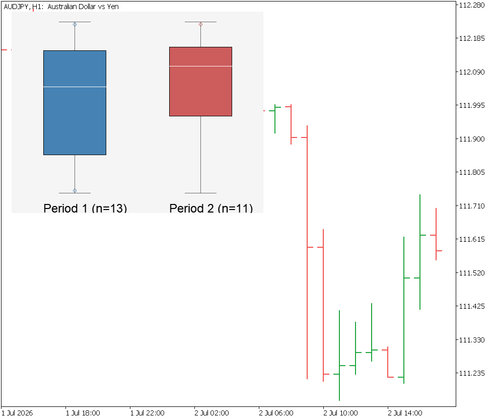
The CCanvas dual box-and-whisker chart rendered by CBoxPlotRenderer::Render() on the AUDJPY, H1 chart, comparing Period 1 (n=13, steel blue) against Period 2 (n=11, Indian red). Each box spans the interquartile range with a white median line, whiskers extend to the most extreme value within the Tukey 1.5×IQR fence, and the small hollow circle above each whisker marks an individual trade classified as an outlier and excluded from the whisker itself. Both boxes render at a comparable, readable size on the shared axis despite the outliers present in each group.

Section 8: Verification

TestMannWhitney.mq5 checks the implementation against a hand-computed example:

Group A = {12, 15, 18, 22, 25}, Group B = {10, 11, 14, 19, 30}. The pooled sorted sequence is: 10(B), 11(B), 12(A), 14(B), 15(A), 18(A), 19(B), 22(A), 25(A), 30(B). No ties exist, so every observation receives a distinct integer rank.

Quantity	Expected Value
R₁ (Group A ranks: 3+5+6+8+9)	31
R₂ (Group B ranks: 1+2+4+7+10)	24
U₁ = 31 − 5·6/2	16
U₂ = 24 − 5·6/2	9
Identity check: U₁ + U₂	25 = 5*5 ✓
U = min(16, 9)	9
z	−0.7311
p	0.4647

The p-value of 0.4647 is well above any conventional alpha, which is expected — these two samples overlap substantially and should fail to reject H₀.

//+------------------------------------------------------------------+
//|                                              TestMannWhitney.mq5 |
//+------------------------------------------------------------------+

#include <MannWhitney\MannWhitneyTest.mqh>

#define ASSERT(cond,msg) { if(cond) Print("PASS: ",msg); else Print("FAIL: ",msg); }

//+------------------------------------------------------------------+
//| Script program start function                                    |
//+------------------------------------------------------------------+
void OnStart(void)
  {
   double groupA[]= {12.0,15.0,18.0,22.0,25.0};
   double groupB[]= {10.0,11.0,14.0,19.0,30.0};

   CMannWhitneyTest test;
   test.SetGroup1(groupA);
   test.SetGroup2(groupB);

   bool ran=test.Run();
   ASSERT(ran==true,"Run() completes successfully");

   double u=test.GetU();
   double z=test.GetZ();
   double p=test.GetP();

   double tol=0.01;

   ASSERT(MathAbs(u-9.0)<tol,
          StringFormat("U statistic equals 9.0 (got %.4f)",u));
   ASSERT(MathAbs(z-(-0.7311))<0.005,
          StringFormat("z-score approximately -0.7311 (got %.4f)",z));
   ASSERT(MathAbs(p-0.4647)<0.005,
          StringFormat("p-value approximately 0.4647 (got %.4f)",p));

   double q1,q2,q3;
   test.ComputeQuartiles(groupA,q1,q2,q3);
   ASSERT(MathAbs(q2-18.0)<tol,
          StringFormat("Group A median equals 18.0 (got %.4f)",q2));
  }
//+------------------------------------------------------------------+

Running TestMannWhitney.mq5 prints five lines to the Experts tab:

PASS: Run() completes successfully
PASS: U statistic equals 9.0 (got 9.0000)
PASS: z-score approximately -0.7311 (got -0.7311)
PASS: p-value approximately 0.4647 (got 0.4647)
PASS: Group A median equals 18.0 (got 18.0000)

Each line points to a different part of the implementation if it fails. A failure on the U statistic line means the problem is in RankPooled() or in the rank-sum arithmetic inside Run(). A failure on the z-score line, with the U statistic still passing, points to the variance formula or the tie correction term. A failure on the p-value line, with a passing z-score, isolates the problem to NormalCDF() specifically, since that is the only additional computation between the two. A failure on the median line points to ComputeQuartiles(), which is otherwise not exercised by the U, z, or p checks.

This structure means a single FAIL line is usually enough to know which method to inspect first, without needing to step through the whole test in a debugger.

Section 9: Interpreting the Output

A concrete example helps ground the interpretation. Suppose the script prints:

U = 214   z = -2.31   p = 0.021

At α = 0.05 this rejects H₀. The two return distributions are distinguishable at a level unlikely to be due to chance alone. The negative z-score indicates that Period 1's rank sum was below the expected value under H₀, meaning Period 2's returns tended to rank higher. The practical question — whether the difference is large enough to act on — requires looking at the box plot medians and computing an effect-size measure such as the Hodges-Lehmann estimator (the median of all n₁×n₂ pairwise differences between the two groups), which uses the same rank machinery already built here.

If instead p = 0.31, the test provides no evidence against treating the two periods as drawn from the same distribution. Pooling the data for further calibration is statistically defensible. Failing to reject H₀ is not the same as concluding the periods are identical; it means the available sample is not large enough to detect a difference, if one exists.

Section 10: Limitations

The normal approximation becomes unreliable below approximately 20 observations per group. Below that threshold, treat the reported p-value as a rough signal rather than a precise probability. An exact permutation-based p-value would be more reliable at small samples.

The test detects any distributional difference, not only a shift in location. Two periods with the same median but different variance or tail shape can produce a significant result. Rejecting H₀ should not be read automatically as "Period A has higher returns" without also inspecting the box plot.

Sequential trades from the same EA are not strictly independent. Consecutive trades can be correlated through shared market conditions, open-position interactions, or intra-window parameter drift. The implementation does not correct for this. The test is best treated as a diagnostic tool rather than a formally airtight inference.

The test reports whether a difference is detectable, not how large it is. The Hodges-Lehmann estimator provides an effect-size companion to this test and reuses the same rank machinery. For comparing three or more regimes simultaneously, the Kruskal-Wallis test generalizes the same ranking procedure to multiple groups.

Conclusion

This article implements a complete, native MQL5 toolkit for comparing trade-return distributions without assuming normality. CMannWhitneyTest handles pooling, ranking with tie correction, U-statistic computation, and p-value derivation via a native normal CDF approximation. CBoxPlotRenderer draws a shared-axis dual box-and-whisker chart with Tukey fence whiskers and outlier markers. MannWhitneyDemo extracts correctly filtered per-trade returns from live history and connects both components.

The key implementation choices that matter in practice are the custom struct sort required by MQL5's ArraySort() limitation, the tie-correction accumulation as a side effect of RankPooled() rather than a separate scan, the intentionally empty destructor that keeps the chart panel visible after the script exits, and the fence-bounded shared axis that prevents a single outlier trade from collapsing either group's box to invisibility.

Programs used in the article:

#	Name	Type	Description
1	MannWhitneyTest.mqh	Include File	Defines the CMannWhitneyTest class that ranks two pooled samples, computes the tie-corrected U statistic and its normal approximation, and reports a p-value and plain-language conclusion.
2	BoxPlotRenderer.mqh	Include File	Defines the CBoxPlotRenderer class that draws a dual box-and-whisker chart for two samples on a shared canvas using CCanvas.
3	MannWhitneyDemo.mq5	Script	Reads closed trade history for two user-defined date ranges, runs the Mann-Whitney test, prints the result, and renders the box-and-whisker comparison on the active chart.
4	TestMannWhitney.mq5	Script	Verifies CMannWhitneyTest against a hand-computed two-group example using an ASSERT macro that prints PASS or FAIL for each checked value.
5	MannWhitney.zip	Zip Archive	Zip archive containing all the attached files and their paths relative to the terminal's root folder.