

Rough Volatility: Building a Roughness Index Feature from the RFSV Model for ML Trade Filtering
 189
189
 0
0

Introduction
Most volatility models you'll find in retail trading circles assume volatility itself moves smoothly — an EWMA here and a GARCH(1,1) there, both built on the idea that today's variance is a gentle blend of yesterday's variance and yesterday's shock. Actual market volatility does not behave that way. Since the 2014 work by Gatheral, Jaisson and Rosenbaum, which introduced what is now called rough volatility, a growing body of empirical evidence has shown that log-volatility itself looks like a fractional Brownian motion with a Hurst exponent far below the standard 0.5 — typically somewhere around 0.05 to 0.15. In plain terms: volatility is "rougher" than a random walk. It jitters and reverts far more locally than a smooth diffusion process would predict.
This article walks through turning that observation into something you can actually use inside an Expert Advisor. We estimate a rolling "roughness index" — a local Hurst exponent — directly from XAUUSD M5 price data using a generalized structure-function regression, implemented natively in MQL5 with no external DLLs or ALGLIB dependency. That roughness index, together with two complementary features, feeds a gradient-boosted classifier trained offline in Python and deployed through ONNX. The EA uses the classifier's output as a standalone directional filter: enter long when the model is confident the regime favors upside, short when it favors downside, and stay flat everywhere in between.
Everything below is working production code. It is the same code shipped in the downloadable archive, not simplified examples. I'll walk through the math first, then the native MQL5 implementation of that math, then the offline training pipeline that has to mirror it bar-for-bar, and finally how the Expert Advisor wires all three pieces together into entries, stops, and position sizing.
One key architectural choice is to compute roughness natively in MQL5. It is not computed offline, streamed in, or delegated to a DLL. A live EA must recompute H_t on every closed bar. It should not rely on external dependencies (which Strategy Tester agents may not access) or on round-trip latency to external processes. Writing the structure-function regression as plain MQL5 accumulator math, rather than reaching for ALGLIB's more general-purpose regression routines, keeps the whole estimator self-contained, auditable line-by-line, and fast enough to run every bar without a second thought.
Scope note: this article documents a real, completed first-pass test of the roughness index as a standalone directional feature — and that first pass lost money in the Strategy Tester. I'm walking through the full system and the honest result together, including why it likely fell short, rather than only publishing once something profitable turns up.
Contents
- Introduction
- Rough Volatility and the RFSV Model
- Estimating the Roughness Index Natively in MQL5
- From Price Stream to Feature Vector
- Training and Exporting the ONNX Classifier
- Wiring the Expert Advisor
- Edge Cases and Pitfalls
- Testing in the Strategy Tester
- Conclusion
Rough Volatility and the RFSV Model
The RFSV (Rough Fractional Stochastic Volatility) model treats log-volatility as a fractional Brownian motion:
log σ t = m + η · BHt
where BH is fractional Brownian motion with Hurst exponent H, m is a long-run mean level, and η controls the amplitude of the fluctuations. When H = 0.5 you get ordinary Brownian motion — the textbook diffusion assumption. What the empirical volatility studies keep finding, across equity indices, FX and commodities alike, is H sitting well under 0.5, often below 0.15. A low H means the path is rougher: it has more high-frequency wiggle and less long-range persistence than a standard random walk, and it tends to mean-revert more sharply after a shock.
The estimation trick that makes this usable comes from the scaling behavior of fractional Brownian motion. For any lag Δ, the expected squared increment scales as a power of the lag:
E[ (log σ t+Δ - log σ t )² ] ∝ Δ2H
Take logs of both sides and this becomes a straight line: log of the expected squared increment against log of the lag has slope exactly 2H. So the estimation procedure is: compute the empirical structure function m(Δ) — the mean squared increment — at a handful of different lags, regress log m(Δ) on log Δ, and read H off as half the slope. That's the entire estimator, and it's the one implemented in both the MQL5 class below and its Python mirror.
One practical issue is that a single M5 close-to-close return is too noisy for log-volatility estimation. It is dominated by microstructure effects and bid/ask bounce rather than underlying volatility. The fix used throughout this system is blocking — accumulate squared log-returns over a small window of bars (six M5 bars, i.e. thirty minutes, by default) into a realized variance estimate, then treat the log of that realized variance as one point in the log-volatility series. This is the same realized-variance-then-log step used in most of the empirical rough-vol literature, just adapted to a bar-based intraday setting instead of daily closes.
Estimator in one sentence: block returns into realized variance → take log → regress log-squared-increments against log-lag across a small ladder of lags → H is half the slope.
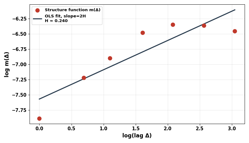
Fig. 1. Log-log structure function m(Δ) plotted against lag Δ for a synthetic rough log-volatility series (true H ≈ 0.10). The regression slope, divided by two, recovers the local Hurst estimate.
Why does this matter as an ML feature rather than just an academic curiosity? A falling roughness index tends to coincide with volatility that is churning and mean-reverting rather than trending — the kind of regime where directional signals are less reliable. A rising, more moderate H, closer to 0.5, is more consistent with smoother, more persistent volatility dynamics, which historically lines up with cleaner trend continuation. The classifier doesn't need to be told this relationship explicitly; it learns whatever structure is actually present in the H-labeled training data, but feeding it a well-motivated, theoretically grounded feature gives it a much better starting point than raw price or a generic volatility measure would.
It's worth being upfront about a simplification made here relative to the academic RFSV literature. The original Gatheral-Jaisson-Rosenbaum estimator fits H from several moments of the log-volatility increments (q = 0.5, 1, 1.5, 2, 3) and regresses the resulting scaling exponents against q, which is more statistically efficient because it pools information across multiple moment orders instead of relying on the variance (q = 2) alone. That multi-moment version is expensive to reproduce bar-by-bar inside MQL5 without a proper linear algebra library, so this implementation uses the single-moment (q = 2) variant of the same scaling relation. The trade-off is a somewhat noisier H estimate in exchange for an estimator that's a few dozen lines of native accumulator math with no external dependency — a reasonable trade for a live feature that has to run on every bar.
Estimating the Roughness Index Natively in MQL5
The estimator lives in CHurstEstimator, a self-contained class with no dependency on ALGLIB or any external DLL — the regression is a handful of accumulator variables and a closed-form OLS slope, which is cheap enough to run every bar without any performance concern. The class keeps its own ring buffer of log-volatility values so the EA never has to manage array indexing directly; it just calls Update() once per completed volatility block and ComputeRoughness() whenever it wants a fresh estimate.
The constant block below defines the shared sizing constants used across the whole include file — the maximum lag-ladder length the estimator will accept, and the fixed input/output width the ONNX classifier expects. Keeping these as named constants rather than magic numbers means the EA, the estimator, and the ONNX wrapper all agree on the same shapes without having to be kept in sync by hand.
//+------------------------------------------------------------------+
//| Includes                                                         |
//+------------------------------------------------------------------+
#include <Trade\Trade.mqh>          // CTrade wrapper used by the EA for order placement

//+------------------------------------------------------------------+
//| Compile-time constants                                           |
//+------------------------------------------------------------------+
#define RFSV_MAX_LAGS      8        // hard ceiling on lag-ladder length used in the structure-function regression
#define RFSV_MODEL_INPUTS  3        // feature count the ONNX classifier expects: H, vol level, vol-of-vol
Here is the full class, exactly as it ships in RFSV_Roughness.mqh. Note the ring-buffer indexing helper RingIndex(): rather than physically shifting the array on every update (which would be O(n) per bar), the buffer is addressed as a circular structure and only the read-out step in ComputeRoughness() linearizes the most recent window into a working array. The constructor seeds m_lastH at 0.5 — the standard-Brownian default — so that if anything ever reads the estimator before it's warmed up, it gets a neutral value rather than an uninitialized one.
In ComputeRoughness(), the code evaluates each lag in the ladder and computes the mean squared increment over valid pairs. It skips lags with fewer than five pairs and lags with non-positive means (to avoid invalid MathLog() inputs). It then computes the OLS slope using four accumulated sums, without intermediate arrays. The Hurst estimate is clamped to [0.01, 0.60] — wide enough to cover anything the empirical literature reports, tight enough to stop a genuinely degenerate window (near-constant volatility, for instance) from handing the classifier an extreme outlier value it never saw in training.
//+------------------------------------------------------------------+
//| CHurstEstimator                                                  |
//+------------------------------------------------------------------+
//| Maintains a rolling buffer of log-volatility observations and    |
//| estimates the local roughness (Hurst exponent H) of that series  |
//| via a generalized structure-function regression:                 |
//|   m(Delta) = mean( (logVol[t] - logVol[t-Delta])^2 )             |
//|   log(m(Delta)) ~= 2H * log(Delta) + const                       |
//| so H is recovered as half the OLS slope of log(m) on log(Delta). |
//| This mirrors the offline Python estimator bar-for-bar so the     |
//| live feature and the training feature are computed identically.  |
//+------------------------------------------------------------------+
class CHurstEstimator
  {
private:
   double            m_logVol[];       // circular buffer of block-level log-volatility values
   int               m_capacity;       // physical size of m_logVol (>= m_window)
   int               m_count;          // number of valid entries currently stored
   int               m_head;           // index where the next value will be written (ring pointer)
   int               m_window;         // regression window length (how many points feed the slope fit)
   int               m_lags[];         // lag ladder (in blocks) used to build the structure function
   int               m_lagCount;       // number of active lags in m_lags
   double            m_lastH;          // most recently computed Hurst estimate
   double            m_lastVolOfVol;   // std-dev of the log-vol series over the regression window

   //+------------------------------------------------------------------+
   //| RingIndex                                                        |
   //+------------------------------------------------------------------+
   int               RingIndex(const int logicalIndex) const
     {
      // logicalIndex counts forward from the oldest retained sample
      int start = (m_head - m_count + m_capacity) % m_capacity;
      return (start + logicalIndex) % m_capacity;
     }

public:
                     CHurstEstimator();
                    ~CHurstEstimator() {};

   bool              Init(const int window,const int &lags[],const int lagCount);
   void              Update(const double newLogVol);
   bool              IsReady() const { return (m_count>=m_window); }
   bool              ComputeRoughness(double &H_out,double &volOfVol_out);
   double            LastH() const { return m_lastH; }
   double            LastVolOfVol() const { return m_lastVolOfVol; }
  };

//+------------------------------------------------------------------+
//| Constructor                                                      |
//+------------------------------------------------------------------+
CHurstEstimator::CHurstEstimator()
  {
   m_capacity     = 0;
   m_count        = 0;
   m_head         = 0;
   m_window       = 0;
   m_lagCount     = 0;
   m_lastH        = 0.5;   // neutral default (standard Brownian) before any data has arrived
   m_lastVolOfVol = 0.0;
  }

//+------------------------------------------------------------------+
//| Init                                                             |
//+------------------------------------------------------------------+
bool CHurstEstimator::Init(const int window,const int &lags[],const int lagCount)
  {
//--- guard: a regression needs more points than the largest lag it tests, otherwise m(Delta) is undefined
   if(window<20 || lagCount<3 || lagCount>RFSV_MAX_LAGS)
      return(false);

   m_window   = window;
//--- buffer is sized generously beyond the window so Update() never has to reallocate mid-run
   m_capacity = window*2;
   ArrayResize(m_logVol,m_capacity);
   ArrayInitialize(m_logVol,0.0);

   m_lagCount = lagCount;
   ArrayResize(m_lags,m_lagCount);
   for(int i=0;i<m_lagCount;i++)
     {
      //--- reject any lag that would exceed the window; such a lag has too few pairs to average reliably
      if(lags[i]<1 || lags[i]>=window)
         return(false);
      m_lags[i]=lags[i];
     }

   m_count = 0;
   m_head  = 0;
   return(true);
  }

//+------------------------------------------------------------------+
//| Update                                                           |
//+------------------------------------------------------------------+
void CHurstEstimator::Update(const double newLogVol)
  {
//--- write into the ring slot, then advance head; overwritten entries simply age out of the window
   m_logVol[m_head]=newLogVol;
   m_head=(m_head+1)%m_capacity;
   if(m_count<m_capacity)
      m_count++;
  }

//+------------------------------------------------------------------+
//| ComputeRoughness                                                 |
//+------------------------------------------------------------------+
bool CHurstEstimator::ComputeRoughness(double &H_out,double &volOfVol_out)
  {
   if(!IsReady())
      return(false);

//--- pull the most recent m_window observations out of the ring buffer into a linear working array
   double series[];
   ArrayResize(series,m_window);
   int offset=m_count-m_window;   // skip older samples beyond the window if the buffer holds more than needed
   for(int i=0;i<m_window;i++)
      series[i]=m_logVol[RingIndex(offset+i)];

//--- accumulate mean and mean-square structure function m(Delta) for every lag in the ladder
   double logDelta[],logM[];
   ArrayResize(logDelta,m_lagCount);
   ArrayResize(logM,m_lagCount);
   int validLags=0;

   for(int L=0;L<m_lagCount;L++)
     {
      int    lag=m_lags[L];
      double sumSq=0.0;
      int    pairs=0;
      for(int t=lag;t<m_window;t++)
        {
         //--- squared increment over this lag; averaging these approximates E[|B^H_t+d - B^H_t|^2] ~ d^(2H)
         double diff=series[t]-series[t-lag];
         sumSq+=diff*diff;
         pairs++;
        }
      if(pairs<5)
         continue; // too few pairs at this lag to trust the average, skip it rather than poison the regression

      double m_delta=sumSq/pairs;
      if(m_delta<=0.0)
         continue; // log() of a non-positive structure function is undefined, guard against a degenerate flat window

      logDelta[validLags]=MathLog((double)lag);
      logM[validLags]=MathLog(m_delta);
      validLags++;
     }

   if(validLags<3)
      return(false); // not enough usable lag points to fit a stable slope

//--- ordinary least squares slope of log(m) on log(Delta): slope = 2H by the RFSV scaling relation
   double sumX=0.0,sumY=0.0,sumXY=0.0,sumXX=0.0;
   for(int i=0;i<validLags;i++)
     {
      sumX+=logDelta[i];
      sumY+=logM[i];
      sumXY+=logDelta[i]*logM[i];
      sumXX+=logDelta[i]*logDelta[i];
     }
   double n=(double)validLags;
   double denom=(n*sumXX-sumX*sumX);
   if(MathAbs(denom)<1e-12)
      return(false); // degenerate regression (all lags collapsed to one x-value), avoid a divide-by-zero

   double slope=(n*sumXY-sumX*sumY)/denom;
   double H=slope/2.0;

//--- clamp to the theoretically sane range; RFSV literature reports H in roughly [0.02, 0.20] empirically,
//--- but noisy windows can produce out-of-range slopes that we cap rather than feed raw into the model
   if(H<0.01) H=0.01;
   if(H>0.60) H=0.60;

//--- vol-of-vol: dispersion of the log-vol series itself over the same window, a complementary regime signal
   double mean=0.0;
   for(int i=0;i<m_window;i++)
      mean+=series[i];
   mean/=m_window;
   double var=0.0;
   for(int i=0;i<m_window;i++)
      var+=(series[i]-mean)*(series[i]-mean);
   var/=(m_window-1);

   H_out        = H;
   volOfVol_out = MathSqrt(var);
   m_lastH        = H_out;
   m_lastVolOfVol = volOfVol_out;
   return(true);
  }
The vol-of-vol — the standard deviation of the log-volatility series itself over the same window — comes back out of the same function as a second output. It's a natural complement to H: two windows can have an identical roughness estimate while one is calm and the other is violently oscillating around its mean, and the classifier benefits from being able to tell those apart.
The ring buffer is sized to 2 * window to avoid reallocations. This reduces ArrayResize() calls on the per-bar path and avoids unnecessary runtime overhead.
From Price Stream to Feature Vector
Between the raw M5 close price and the Hurst estimator sits CRFSVFeatureEngine, whose job is entirely about turning a stream of per-bar log-returns into the block-level log-volatility observations the estimator consumes, and then assembling the three-element feature vector the ONNX model expects. This separation matters: the estimator class knows nothing about bars, blocks, or trading — it only knows about a generic log-volatility series — while the feature engine owns all of the market-data-specific bookkeeping.
OnBarReturn() is called once per closed bar from the EA's OnTick(). It accumulates squared log-returns into m_sumSqReturns, and once m_blockSize bars have been seen (six, by default, for a thirty-minute block on M5), it computes the block's realized variance, floors it at 1e-14 to guard against a mathematically impossible zero-variance block feeding a log(0) into the next step, takes half the log of that variance to get the block's log-volatility, and pushes it into the Hurst estimator before resetting the accumulator for the next block.
//+------------------------------------------------------------------+
//| CRFSVFeatureEngine                                               |
//+------------------------------------------------------------------+
//| Converts a stream of per-bar log-returns into the block-level    |
//| log-volatility series the Hurst estimator needs, then exposes a  |
//| ready-to-run feature vector for the ONNX classifier.             |
//| Blocking (default 6 M5 bars = 30 minutes) trades granularity for |
//| a realized-variance estimate that is not dominated by bid/ask    |
//| bounce on a single 5-minute bar.                                 |
//+------------------------------------------------------------------+
class CRFSVFeatureEngine
  {
private:
   CHurstEstimator   m_hurst;             // roughness estimator fed by completed volatility blocks
   int               m_blockSize;         // number of bars accumulated per volatility block
   int               m_barInBlock;        // bars accumulated so far in the current, unfinished block
   double            m_sumSqReturns;      // running sum of squared log-returns within the current block
   double            m_prevH;             // H from the previous completed block, used to derive H momentum

public:
                     CRFSVFeatureEngine();
                    ~CRFSVFeatureEngine() {};

   bool              Init(const int hurstWindow,const int &lags[],const int lagCount,const int blockSize);
   void              OnBarReturn(const double logReturn);
   bool              IsReady() const { return(m_hurst.IsReady()); }
   bool              BuildFeatureVector(float &features[]);
  };

//+------------------------------------------------------------------+
//| Constructor                                                      |
//+------------------------------------------------------------------+
CRFSVFeatureEngine::CRFSVFeatureEngine()
  {
   m_blockSize    = 6;      // default: 6 x M5 bars = 30-minute volatility blocks
   m_barInBlock   = 0;
   m_sumSqReturns = 0.0;
   m_prevH        = 0.5;
  }

//+------------------------------------------------------------------+
//| Init                                                             |
//+------------------------------------------------------------------+
bool CRFSVFeatureEngine::Init(const int hurstWindow,const int &lags[],const int lagCount,const int blockSize)
  {
   if(blockSize<1)
      return(false);
   m_blockSize = blockSize;
//--- delegate the regression-window and lag-ladder validation to the estimator itself
   return(m_hurst.Init(hurstWindow,lags,lagCount));
  }

//+------------------------------------------------------------------+
//| OnBarReturn                                                      |
//+------------------------------------------------------------------+
void CRFSVFeatureEngine::OnBarReturn(const double logReturn)
  {
//--- accumulate squared return; this is the realized-variance building block for the current volatility block
   m_sumSqReturns += logReturn*logReturn;
   m_barInBlock++;

   if(m_barInBlock>=m_blockSize)
     {
      //--- realized variance over the block, floored to avoid log(0) on a completely flat block
      double realizedVar=MathMax(m_sumSqReturns,1e-14);
      //--- log-volatility = 0.5 * log(realized variance); this is the series the RFSV model treats as fBm
      double logVol=0.5*MathLog(realizedVar);
      m_hurst.Update(logVol);

      //--- reset the block accumulator for the next window of bars
      m_sumSqReturns = 0.0;
      m_barInBlock   = 0;
     }
  }

//+------------------------------------------------------------------+
//| BuildFeatureVector                                               |
//+------------------------------------------------------------------+
bool CRFSVFeatureEngine::BuildFeatureVector(float &features[])
  {
   double H,volOfVol;
   if(!m_hurst.ComputeRoughness(H,volOfVol))
      return(false);

//--- H momentum: how fast the local roughness is shifting block-to-block, a leading regime-change signal
   double hMomentum=H-m_prevH;
   m_prevH=H;

   ArrayResize(features,RFSV_MODEL_INPUTS);
   features[0]=(float)H;          // roughness index — lower H implies rougher, more mean-reverting volatility
   features[1]=(float)volOfVol;   // dispersion of log-vol over the window — regime turbulence proxy
   features[2]=(float)hMomentum;  // directional drift of the roughness estimate itself
   return(true);
  }
BuildFeatureVector() is the last stop before the ONNX call. Besides pulling H and vol-of-vol out of the estimator, it computes a third feature — H momentum, the change in H from the previous completed block to the current one. This is deliberately not something the Hurst estimator itself tracks, since momentum is a property of the sequence of estimates rather than of any single window; keeping it in the feature engine keeps the estimator class focused purely on estimation. A roughness index that's falling fast tells a different story than one that's been flat at the same low value for hours, and giving the classifier that derivative directly, rather than making it infer it from consecutive raw H values across separate calls, produces a materially cleaner training signal.
Training and Exporting the ONNX Classifier
The offline half of this system lives in rfsv_train_export.py, and the single most important design constraint on it is that it has to reproduce the MQL5 math exactly — not approximately, not "close enough," but the same accumulation order, same clamps, same floor values. Any drift between the two implementations means the classifier is scored on features it was never actually trained on once it hits a live chart. The configuration block at the top mirrors the EA's input parameters one-for-one, including the exact lag ladder, so a change to one side is a visible, deliberate change that has to be mirrored on the other.
# --------------------------------------------------------------------- #
# Configuration - mirrors the EA's input parameters exactly             #
# --------------------------------------------------------------------- #
HURST_WINDOW   = 100            # regression window, in completed volatility blocks
BLOCK_SIZE     = 6              # M5 bars per volatility block (30 minutes)
LAG_LADDER     = [1, 2, 3, 5, 8, 13]  # must match InpLag1..InpLag6 in the EA
compute_block_log_vol() is the direct counterpart to OnBarReturn()'s blocking logic — same six-bar block size by default, same realized-variance floor, same 0.5 × log(variance) transform:
HISTORY_DAYS   = 240            # how many calendar days of M5 history to pull
ONNX_OUT_PATH  = "rfsv_classifier.onnx"

def fetch_mt5_history(symbol: str, timeframe, days: int) -> pd.DataFrame:
    """Connect to the running MT5 terminal and pull M5 OHLC history directly.

    Replaces the old manual "export to CSV from the chart" step entirely -
    this talks to the same running terminal you're logged into.
    """
    if not mt5.initialize():
        raise RuntimeError(
            f"mt5.initialize() failed, error = {mt5.last_error()}. "
            "Make sure the MT5 terminal is open and you are logged in."
rolling_hurst() mirrors ComputeRoughness() almost line for line: same lag ladder, same "skip if fewer than five pairs" guard, same non-positive-mean guard, same OLS normal-equations formulation, same H = slope / 2 relation, same [0.01, 0.60] clamp. Where the MQL5 version updates a rolling estimate incrementally bar-by-bar, this Python version recomputes the regression fresh for every window end-point across the whole historical series — slower, but appropriate for an offline batch job building a training set rather than a live per-tick calculation.
# confirm the symbol exists and is visible in Market Watch, add it if not
    info = mt5.symbol_info(symbol)
    if info is None:
        mt5.shutdown()
        raise RuntimeError(
            f"Symbol '{symbol}' not found. Check the exact spelling in Market "
            "Watch - some brokers use suffixes like XAUUSD.m or XAUUSDm."
        )
    if not info.visible:
        mt5.symbol_select(symbol, True)

    utc_to = datetime.now()
    utc_from = utc_to - timedelta(days=days)
    rates = mt5.copy_rates_range(symbol, timeframe, utc_from, utc_to)
    mt5.shutdown()

    if rates is None or len(rates) == 0:
        raise RuntimeError(
            f"No rates returned for {symbol}. Check that the symbol has "
            "enough history available in the terminal (scroll back on its "
            "chart at least once so the terminal caches the history)."
        )

    df = pd.DataFrame(rates)
    df["time"] = pd.to_datetime(df["time"], unit="s")
    df = df.sort_values("time").reset_index(drop=True)
    print(f"fetched {len(df)} M5 bars for {symbol}, "
          f"{df['time'].iloc[0]} -> {df['time'].iloc[-1]}")
    return df

def compute_block_log_vol(close: np.ndarray, block_size: int) -> np.ndarray:
    """Convert a closed-bar close-price series into block-level log-volatility.

    Mirrors CRFSVFeatureEngine::OnBarReturn(): accumulate squared log-returns
    over `block_size` bars, then log_vol = 0.5 * log(realized_variance).
    """
    log_returns = np.diff(np.log(close))
    n_blocks = len(log_returns) // block_size
    log_vol = np.empty(n_blocks)
    for i in range(n_blocks):
        block = log_returns[i * block_size:(i + 1) * block_size]
        realized_var = max(np.sum(block ** 2), 1e-14)  # same floor as the MQL5 guard
        log_vol[i] = 0.5 * np.log(realized_var)
    return log_vol
build_feature_frame() assembles the three-column feature matrix and attaches the training label: the sign of the forward block-level return, twelve blocks (six hours) ahead by default. Using a forward-looking label computed strictly from data after the feature window, combined with the chronological (non-shuffled) train/test split further down in main(), keeps the whole pipeline free of look-ahead leakage.
 """Rolling structure-function Hurst estimate, one output per completed window.

    This is the direct counterpart of CHurstEstimator::ComputeRoughness():
    for each lag, average the squared increment over the window, regress
    log(mean_sq_increment) on log(lag) via OLS, and take H = slope / 2.
    Returns (H_series, vol_of_vol_series), both aligned to the *end* of
    each window (i.e. index i corresponds to log_vol[i - window + 1 : i+1]).
    """
    n = len(log_vol)
    H_out = np.full(n, np.nan)
    vv_out = np.full(n, np.nan)

    for end in range(window - 1, n):
        series = log_vol[end - window + 1: end + 1]

        log_delta, log_m = [], []
        for lag in lags:
            diffs = series[lag:] - series[:-lag]
            if len(diffs) < 5:
                continue  # same "too few pairs" guard as the MQL5 estimator
            m_delta = np.mean(diffs ** 2)
            if m_delta <= 0.0:
                continue
            log_delta.append(np.log(lag))
            log_m.append(np.log(m_delta))
Training uses GradientBoostingClassifier with shallow trees and conservative hyperparameters. The export step addresses two ONNX issues: zipmap output format and the default two-output classifier export. The script disables zipmap and adds a Gather node to output P(class=1) as a [1,1] tensor.
def main():
    # pulls M5 bars straight from the running MT5 terminal — see fetch_mt5_history() above
    df = fetch_mt5_history(SYMBOL, TIMEFRAME, HISTORY_DAYS)

    # build_feature_frame() runs the MQL5-mirrored Hurst/blocking math and attaches the
    # forward-return label; only the three model inputs and the label survive into X/y
    frame = build_feature_frame(df)
    X = frame[["H", "vol_of_vol", "H_momentum"]].to_numpy(dtype=np.float32)
    y = frame["label"].to_numpy()

    # shuffle=False keeps the split chronological: the test set is strictly the most
    # recent 25% of history, so no future information leaks into training via a
    # randomly-shuffled window that straddles both sides of the split
    X_train, X_test, y_train, y_test = train_test_split(
        X, y, test_size=0.25, shuffle=False
    )

    # shallow trees + a conservative learning rate + row subsampling: deliberately
    # conservative defaults, since a 3-feature model has little room to overfit safely
    clf = GradientBoostingClassifier(
        n_estimators=200,
        max_depth=3,
        learning_rate=0.05,
        subsample=0.8,
        random_state=42,
    )
    clf.fit(X_train, y_train)

    # test accuracy on the chronological holdout is the real signal here — if it's
    # not clearly above 0.5, the feature set has no business generating live trades
    train_acc = clf.score(X_train, y_train)
    test_acc = clf.score(X_test, y_test)
    print(f"train accuracy: {train_acc:.4f}  test accuracy: {test_acc:.4f}")

    # ---- ONNX export ---------------------------------------------------
    # float_input / [1,3] must match RFSV_MODEL_INPUTS and the OnnxSetInputShape()
    # call in COnnxRoughnessModel::Init() — a mismatch here fails silently at
    # runtime rather than at export time, so the shape is fixed explicitly
    initial_type = [("float_input", FloatTensorType([1, 3]))]
    onnx_model = convert_sklearn(
        clf,
        initial_types=initial_type,
        target_opset=13,
        # zipmap=False: without this, skl2onnx wraps the probability output in a
        # dictionary-like "zipmap" structure that OnnxRun() cannot consume as a
        # plain matrix<float> — stripping it here avoids a runtime failure later
        options={id(clf): {"zipmap": False}},
    )

    graph = onnx_model.graph
    # a default sklearn classifier export produces two outputs: graph.output[0] is
    # the predicted label, graph.output[1] is the [1,2] probability tensor
    # (columns are P(class=0), P(class=1)); the EA only ever wants P(class=1),
    # so the label output is dropped outright rather than carried through unused
    prob_output = graph.output[1]
    prob_output.name = "probabilities"
    del graph.output[0]

    # RFSV_MODEL_OUTPUTS is fixed at 1 on the MQL5 side, so the [1,2] probability
    # tensor still has to be sliced down to a single [1,1] column before saving —
    # a Gather node picks out index 1 (P(class=1)) directly inside the graph,
    # which keeps the slicing baked into the .onnx file instead of relying on the
    # MQL5 caller to know which column to read
    from onnx import helper, TensorProto
    gather_indices = helper.make_tensor("gather_idx", TensorProto.INT64, [1], [1])
    graph.initializer.append(gather_indices)
    gather_node = helper.make_node(
        "Gather",
        inputs=["probabilities", "gather_idx"],
        outputs=["prob_up"],
        axis=1,
        name="SelectClass1Probability",
    )
    graph.node.append(gather_node)
    # replace the now-stale [1,2] output declaration with the true [1,1] shape
    # the Gather node actually produces — leaving the old declaration in place
    # would make the graph internally inconsistent and fail onnx.checker below
    graph.output[0].CopyFrom(
        helper.make_tensor_value_info("prob_up", TensorProto.FLOAT, [1, 1])
    )

    # validates the graph is well-formed (correct shapes, no dangling nodes)
    # before it's trusted enough to write to disk and embed into the EA
    onnx.checker.check_model(onnx_model)
    with open(ONNX_OUT_PATH, "wb") as f:
        f.write(onnx_model.SerializeToString())

    print(f"saved {ONNX_OUT_PATH}")
    print(f"  opset: {onnx_model.opset_import[0].version}")
    print(f"  ir_version: {onnx_model.ir_version}")
    print(f"  input: float_input, shape [1,3] -> [H, vol_of_vol, H_momentum]")
    print(f"  output: prob_up, shape [1,1] -> P(forward return > 0)")
The Gather node deserves a closer look since it's the least obvious part of the export. Rather than leaving "read column 1 of the probability tensor" as something the MQL5 caller has to know and get right, the node bakes that slicing directly into the saved graph — the .onnx file itself outputs a single float named prob_up, so there's no column-selection convention that could get out of sync between the Python export and the MQL5 wrapper. The onnx.checker.check_model() call right before saving exists specifically to catch a graph left in an inconsistent state by this kind of manual surgery — if the output shape declaration and what the Gather node actually produces ever drifted apart, this is where it would be caught, at export time on a developer's machine, rather than as a silent runtime failure inside OnnxRun() on a live chart.
The exported artifact, rfsv_classifier.onnx, has an opset of 13, an IR version set by whichever onnx package version performed the export, one input tensor named float_input with shape [1, 3] mapping to [H, vol_of_vol, H_momentum] in that exact order, and one output tensor named prob_up with shape [1, 1]. That file needs to be copied to MQL5\Files\RFSV_Roughness\rfsv_classifier.onnx in the terminal's data folder before compiling the EA, since it's pulled in at compile time through a #resource directive rather than read from disk at runtime.
On the train/test split and metric side: main() deliberately uses shuffle=False in train_test_split, holding out the most recent 25% of the labeled history as a chronological test set rather than a randomly shuffled one. Financial time series data is autocorrelated, and a shuffled split would let information from test-period volatility blocks leak into the training set through overlapping windows, producing an inflated accuracy number that won't survive contact with a live chart. The train/test accuracy printed at the end of the script is a sanity check, not a performance guarantee — a classifier that's only marginally better than the roughly 50% base rate on a chronological, non-shuffled split is still worth testing inside the EA, since even a small, persistent edge compounds meaningfully once it's combined with disciplined position sizing and risk management.
Wiring the Expert Advisor
The EA, RFSV_Roughness_EA.mq5, is deliberately thin — almost everything interesting already happened in the include file's three classes. Its job is initialization, the new-bar loop, and turning a probability into an order. The resource directive at the top embeds the ONNX file directly into the compiled .ex5, which sidesteps a recurring Strategy Tester issue: each tester agent runs with its own isolated Files folder, so an ONNX model that's only present on disk in the terminal's main data folder won't be visible to optimization agents. Embedding it as a resource means the model travels with the compiled program itself.
//+------------------------------------------------------------------+
//| Resources                                                        |
//+------------------------------------------------------------------+
#resource "\\Files\\RFSV_Roughness\\rfsv_classifier.onnx" as uchar ModelBuffer[]
// embedding the model as a resource means the Strategy Tester's isolated agent
// sandbox always finds it, sidestepping the Files-folder-per-agent limitation

//+------------------------------------------------------------------+
//| Input parameters — Hurst / RFSV feature engine                   |
//+------------------------------------------------------------------+
input int    InpHurstWindow   = 100;    // Hurst regression window, in completed volatility blocks
input int    InpBlockSize     = 6;      // M5 bars per volatility block (6 = 30 minutes)
input int    InpLag1          = 1;      // lag ladder point 1 (blocks)
input int    InpLag2          = 2;      // lag ladder point 2 (blocks)
input int    InpLag3          = 3;      // lag ladder point 3 (blocks)
input int    InpLag4          = 5;      // lag ladder point 4 (blocks)
input int    InpLag5          = 8;      // lag ladder point 5 (blocks)
input int    InpLag6          = 13;     // lag ladder point 6 (blocks)

//+------------------------------------------------------------------+
//| Input parameters — classifier gating                             |
//+------------------------------------------------------------------+
input double InpProbLongAbove  = 0.60;  // enter long when P(up) exceeds this
input double InpProbShortBelow = 0.40;  // enter short when P(up) falls below this

//+------------------------------------------------------------------+
//| Input parameters — risk & trade management                       |
//+------------------------------------------------------------------+
input int    InpATRPeriod      = 14;    // ATR period used for sizing and stops
input double InpATRMultSL      = 2.0;   // stop-loss distance as a multiple of ATR
input double InpATRMultTP      = 3.0;   // take-profit distance as a multiple of ATR
input double InpRiskPercent    = 0.5;   // percent of account equity risked per trade
input ulong  InpMagicNumber    = 20260901; // magic number identifying this EA's positions
Globals hold one instance each of the feature engine, the ONNX wrapper, and the trade helper, plus the ATR handle used for both stop distances and position sizing:
//+------------------------------------------------------------------+
//| Globals — engine, model, trading, indicator handles              |
//+------------------------------------------------------------------+
CRFSVFeatureEngine g_engine;      // computes H_t, vol-of-vol, H-momentum from the live price stream
COnnxRoughnessModel g_model;      // wraps the resource-embedded ONNX classifier
CTrade             g_trade;       // standard trade wrapper for order placement
int                g_atrHandle;   // handle for the ATR indicator used in sizing/stops
datetime           g_lastBarTime; // timestamp of the last bar processed, used for the new-bar guard
OnInit() assembles the lag ladder from the six individually-tunable inputs (so each lag can be optimized independently in the Strategy Tester rather than being locked into a hard-coded array), then initializes the feature engine, loads the ONNX model from the embedded resource buffer, and creates the ATR handle. Every one of those three steps can fail independently — a bad window/lag combination, a corrupted or mismatched ONNX export, or a symbol the terminal can't build an ATR series for — and each failure returns a distinct, logged initialization code rather than falling through to a generic failure, which makes diagnosing a failed load in the Experts log far faster than a single catch-all return would.
//+------------------------------------------------------------------+
//| Expert initialization function                                   |
//+------------------------------------------------------------------+
int OnInit()
  {
//--- assemble the lag ladder from individual inputs so each lag is independently tunable/optimizable
   int lags[6];
   lags[0]=InpLag1; lags[1]=InpLag2; lags[2]=InpLag3;
   lags[3]=InpLag4; lags[4]=InpLag5; lags[5]=InpLag6;

   if(!g_engine.Init(InpHurstWindow,lags,6,InpBlockSize))
     {
      //--- fail fast: a misconfigured window/lag combination would silently produce garbage H estimates
      Print("RFSV_Roughness_EA: feature engine Init failed — check window/lag inputs");
      return(INIT_PARAMETERS_INCORRECT);
     }

   if(!g_model.Init(ModelBuffer))
     {
      //--- the embedded resource is the only model source; if it fails to load there is nothing to fall back to
      Print("RFSV_Roughness_EA: ONNX model Init failed — verify rfsv_classifier.onnx export");
      return(INIT_FAILED);
     }

   g_atrHandle=iATR(_Symbol,_Period,InpATRPeriod);
   if(g_atrHandle==INVALID_HANDLE)
     {
      Print("RFSV_Roughness_EA: iATR handle creation failed");
      return(INIT_FAILED);
     }

   g_trade.SetExpertMagicNumber(InpMagicNumber);
   g_trade.SetTypeFillingBySymbol(_Symbol);

   g_lastBarTime = 0;
   g_prevClose   = 0.0;

   return(INIT_SUCCEEDED);
  }
OnDeinit() is short but not optional: both the ATR indicator handle and the ONNX session need to be released explicitly. This matters more than it looks like it should, because the Strategy Tester can cycle OnInit()/OnDeinit() repeatedly within a single agent process during optimization runs, and an ONNX session that's never released will leak across those cycles.
//+------------------------------------------------------------------+
//| Expert deinitialization function                                 |
//+------------------------------------------------------------------+
void OnDeinit(const int reason)
  {
//--- release both the indicator handle and the ONNX session explicitly; relying on GC here is unsafe
//--- across Strategy Tester runs where OnDeinit/OnInit can cycle repeatedly within one agent process
   if(g_atrHandle!=INVALID_HANDLE)
      IndicatorRelease(g_atrHandle);
   g_model.Release();
  }
Two small helper functions carry real weight. IsNewBar() gates every meaningful computation in the EA to once per closed bar — the feature engine and classifier are both bar-level constructs, and evaluating them intrabar would just repeat the same work with the same inputs. CalculatePositionSize() converts the ATR-based stop-loss distance into a lot size sized to risk a fixed percentage of equity, with explicit guards against a zero or misreporting tick size/value (which would otherwise divide by zero) and a final snap to the broker's lot step so the resulting order volume is never rejected for an invalid increment.
//+------------------------------------------------------------------+
//| IsNewBar — true exactly once per closed bar                      |
//+------------------------------------------------------------------+
bool IsNewBar()
  {
   datetime currentBarTime=iTime(_Symbol,_Period,0);
   if(currentBarTime!=g_lastBarTime)
     {
      g_lastBarTime=currentBarTime;
      return(true);
     }
   return(false);
  }

//+------------------------------------------------------------------+
//| CalculatePositionSize — risk-percent sizing off the ATR stop     |
//+------------------------------------------------------------------+
double CalculatePositionSize(const double slDistancePrice)
  {
   double equity=AccountInfoDouble(ACCOUNT_EQUITY);
   double riskAmount=equity*(InpRiskPercent/100.0);

   double tickValue=SymbolInfoDouble(_Symbol,SYMBOL_TRADE_TICK_VALUE);
   double tickSize=SymbolInfoDouble(_Symbol,SYMBOL_TRADE_TICK_SIZE);
   if(tickSize<=0.0 || tickValue<=0.0)
      return(0.0); // guard against a misreporting symbol; sizing off a zero denominator would blow up

//--- convert the ATR-based price distance into a monetary loss-per-lot, then solve for lot size
   double lossPerLot=(slDistancePrice/tickSize)*tickValue;
   if(lossPerLot<=0.0)
      return(0.0);

   double rawLots=riskAmount/lossPerLot;

   double minLot =SymbolInfoDouble(_Symbol,SYMBOL_VOLUME_MIN);
   double maxLot =SymbolInfoDouble(_Symbol,SYMBOL_VOLUME_MAX);
   double lotStep=SymbolInfoDouble(_Symbol,SYMBOL_VOLUME_STEP);

//--- snap to the broker's lot step so the order is not rejected for an invalid volume increment
   double lots=MathFloor(rawLots/lotStep)*lotStep;
   lots=MathMax(minLot,MathMin(maxLot,lots));
   return(lots);
  }
OnTick() ties everything together: on each new bar it computes the log-return of the just-closed bar, feeds it to the feature engine, and — once the engine has enough history to produce a real estimate — builds the feature vector and runs the ONNX prediction. It refuses to stack positions (one open position per symbol/magic at a time), pulls the current ATR value for sizing and stops, and only sends an order when the predicted probability clears one of the two configurable thresholds; anything in between is treated as "no edge" and left flat rather than forced into a low-conviction trade.
One design decision worth being explicit about: this version uses the classifier's probability as a standalone directional signal rather than as a filter layered on top of a separate base strategy (a moving-average cross, say, or a breakout rule). That keeps the system easy to reason about end to end — there's exactly one source of directional opinion, and every trade the EA takes can be traced back to a single probability number. The trade-off is that the classifier is carrying the entire directional decision on its own, with no independent signal to cross-check it against. Wiring the same probability output in as a gate on top of an existing base signal instead — only taking the base signal's trades when the classifier agrees — is a straightforward modification if you'd rather use the roughness index that way; the COnnxRoughnessModel::Predict() call and its probability output don't need to change at all, only the entry logic inside OnTick().
//+------------------------------------------------------------------+
//| Expert tick function                                             |
//+------------------------------------------------------------------+
void OnTick()
  {
   if(!IsNewBar())
      return; // the feature engine and classifier are both bar-level, evaluating intrabar would just repeat work

   double closePrice=iClose(_Symbol,_Period,1); // last fully closed bar
   if(g_prevClose<=0.0)
     {
      //--- first call after init has no prior close to diff against; seed it and wait for the next bar
      g_prevClose=closePrice;
      return;
     }

//--- log-return of the just-closed bar feeds the block-level realized-variance accumulator
   double logReturn=MathLog(closePrice/g_prevClose);
   g_prevClose=closePrice;
   g_engine.OnBarReturn(logReturn);

   if(!g_engine.IsReady())
      return; // still filling the initial Hurst regression window, nothing to trade on yet

   float features[];
   if(!g_engine.BuildFeatureVector(features))
      return; // regression could not be fit this bar (degenerate window), skip rather than trade on stale data

   double probUp;
   if(!g_model.Predict(features,probUp))
     {
      Print("RFSV_Roughness_EA: ONNX Predict failed on bar ",TimeToString(g_lastBarTime));
      return;
     }

//--- do not stack positions: only evaluate new entries when flat on this symbol/magic combination
   if(PositionSelect(_Symbol))
      return;

   double atrBuffer[];
   ArraySetAsSeries(atrBuffer,true);
   if(CopyBuffer(g_atrHandle,0,1,1,atrBuffer)<1)
      return; // ATR not yet available (e.g. right after init), skip this bar rather than trade without a stop

   double atr=atrBuffer[0];
   double slDistance=atr*InpATRMultSL;
   double tpDistance=atr*InpATRMultTP;
   if(slDistance<=0.0)
      return;

   double lots=CalculatePositionSize(slDistance);
   if(lots<=0.0)
      return; // sizing degenerated to zero (e.g. equity/tick data unavailable), do not send a zero-volume order

   double ask=SymbolInfoDouble(_Symbol,SYMBOL_ASK);
   double bid=SymbolInfoDouble(_Symbol,SYMBOL_BID);

   if(probUp>InpProbLongAbove)
     {
      //--- classifier favors an upward regime with enough margin above the threshold to act on
      double sl=ask-slDistance;
      double tp=ask+tpDistance;
      g_trade.Buy(lots,_Symbol,ask,sl,tp,"RFSV roughness long");
     }
   else if(probUp<InpProbShortBelow)
     {
      //--- symmetric downside case: classifier favors a downward regime
      double sl=bid+slDistance;
      double tp=bid-tpDistance;
      g_trade.Sell(lots,_Symbol,bid,sl,tp,"RFSV roughness short");
     }
//--- probUp between the two thresholds is treated as "no edge" and intentionally left flat
  }
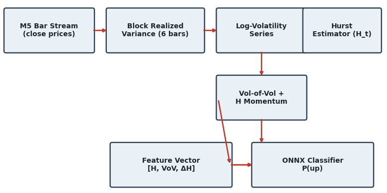
Fig. 2. End-to-end data flow: the M5 bar stream feeds block-level realized variance, which becomes the log-volatility series consumed by the Hurst estimator; H, vol-of-vol and H-momentum form the feature vector passed into the ONNX classifier, whose probability output drives the EA's entry logic.
Edge Cases and Pitfalls
The warm-up period is the first thing to get right when testing this system. CHurstEstimator::IsReady() won't return true until the ring buffer holds a full regression window's worth of blocks — at the defaults (100-block window, six bars per block) that's 600 M5 bars, fifty hours of trading time, before the EA will place its first trade on a fresh chart or in a fresh Strategy Tester run. This isn't a bug to work around; it's the estimator refusing to hand back a regression fit on insufficient data, which is exactly the behavior you want from it.
A flat, near-zero-volatility window is the other scenario the estimator has to defend against explicitly. If price genuinely doesn't move for an extended stretch (illiquid session opens, certain holiday sessions), the realized variance for a block can be numerically indistinguishable from zero, and without the 1e-14 floor in OnBarReturn(), the subsequent MathLog() call would either error or return negative infinity, silently corrupting every downstream Hurst estimate that includes that block in its window.
Watch the recurring MQL5/ONNX pitfalls that show up across this whole article series, all of which apply here too: matrix without an explicit type parameter defaults to matrix<double>, which will not satisfy an ONNX session running in ONNX_NO_CONVERSION mode — both the input and output matrices in COnnxRoughnessModel::Predict() are explicitly typed matrix<float> for exactly this reason. The output matrix also has to be pre-sized to [1, 1] before calling OnnxRun(); an unsized output matrix in no-conversion mode fails silently rather than auto-resizing the way it would in the default conversion mode. And skl2onnx's default double-output behavior (label plus zipmapped probabilities) is a trap if you export without stripping it — the Python script's Gather-node surgery exists specifically to avoid shipping an ONNX file whose output shape doesn't match what the MQL5 wrapper is configured to expect.
One more subtlety worth flagging: the lag ladder itself has to stay well inside the regression window. The Init() guard on CHurstEstimator rejects any lag greater than or equal to the window size, but even a lag that technically passes that check — say, a lag of 90 inside a 100-block window — leaves only ten valid pairs to average, which is barely enough to be numerically stable and nowhere near enough to be statistically trustworthy. The default ladder (1, 2, 3, 5, 8, 13) stays comfortably below the 100-block default window for exactly this reason; widen the window before you widen the ladder, not the other way around.
Position sizing has its own quiet failure mode worth calling out separately from the Hurst estimator: CalculatePositionSize() pulls SYMBOL_TRADE_TICK_VALUE and SYMBOL_TRADE_TICK_SIZE directly from the symbol, which for XAUUSD can vary meaningfully between brokers depending on contract specification and account currency. The function already guards against either value coming back as zero or negative, but it's worth actually checking those two values in the Market Watch symbol specification for your own broker before trusting the resulting lot size on a live account — a specification mismatch won't throw an error, it'll just size positions incorrectly, which is a far harder problem to notice than an outright crash.
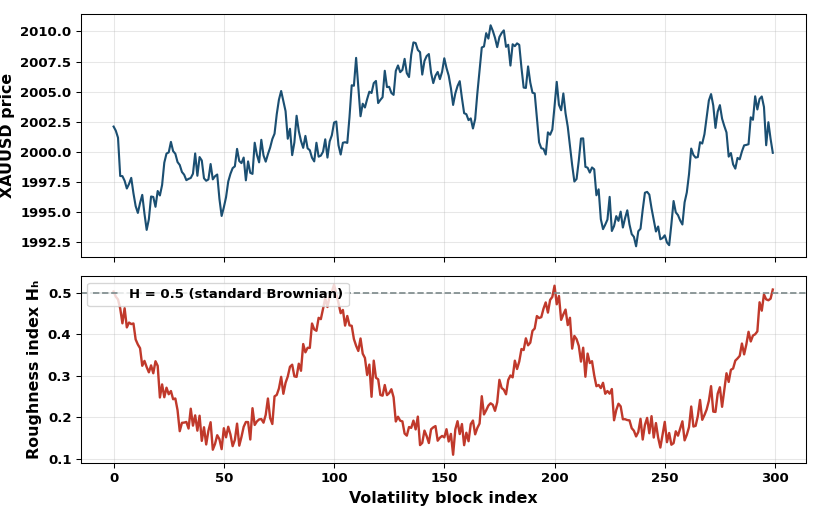
Fig. 3. Synthetic illustration of the rolling roughness index Hₔ tracked alongside price across a series of volatility blocks, with the H = 0.5 standard-Brownian reference line marked for comparison.
Testing in the Strategy Tester
The table below reflects an actual completed Strategy Tester run, not a projection. It was run against the article's default input parameters — no optimization pass, no parameter tuning — on the OHLC (1-minute) tester model, XAUUSD M5, roughly June 3 through August 20, 2026, starting from a $10,000 deposit. I'm reporting it exactly as it came out, including the fact that it lost money, because that's a more useful result for readers than a cherry-picked one.
| Metric | Value |
|---|---|
| Symbol/Timeframe | XAUUSD / M5 |
| Test period | 2026.06.03 – 2026.08.20 (OHLC 1-minute model) |
| Initial deposit | $10,000.00 |
| Total net profit | -$1,262.49 |
| Profit factor | 0.91 |
| Expected payoff | -2.71 per trade |
| Sharpe ratio | -3.36 |
| Max balance drawdown | 27.25% ($3,252.63) |
| Total trades/profitable | 466 trades, 37.34% profitable |
| Long/short win rate | 32.08% long, 40.07% short |
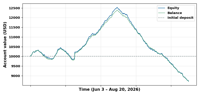
Fig. 4. Balance and equity curve reconstructed from the Strategy Tester's Graph tab for the June–August 2026 run: a climb toward roughly $12,070 by early July, followed by a sustained drawdown to around $8,700–8,800 by August 20, closing at a net loss.
This result isn't a surprise in hindsight — it's consistent with what the offline training run already showed. The gradient-boosted classifier scored 67.82% accuracy on its training data but only 48.03% on the chronological held-out test set, which is worse than a coin flip on a binary up/down label. A model that can't beat random guessing out of sample has no business generating real trade signals, and the Strategy Tester result here is that offline warning made concrete: a profit factor of 0.91, a negative Sharpe ratio, and a win rate under 40% on both sides of the book.
Three features (H, vol-of-vol, H-momentum) and a stock GradientBoostingClassifier configuration is a reasonable starting point for a first pass, not a finished system, and this run is exactly the kind of honest negative result that first pass should produce if the underlying relationship isn't there yet, or isn't there with this feature set. Worth trying before writing off the roughness index entirely: fewer estimators and shallower trees to fight the overfitting gap directly, a longer and more diverse training window than the roughly eight months pulled here, a shorter or asymmetric forward-labeling horizon, and layering the roughness index in as a filter on top of an independent base signal rather than asking it to carry full directional weight on its own, per the alternative wiring already discussed in the previous section.
Conclusion
The honest summary of this first pass: the roughness index is theoretically well-motivated, the native MQL5 estimator and its Python mirror stayed in exact lockstep, the ONNX export and MQL5 inference pipeline worked correctly end to end — and the resulting classifier still lost money in a real Strategy Tester run, with a profit factor of 0.91 and a negative Sharpe ratio over a June–August 2026 test. That's a legitimate outcome of doing this kind of research properly rather than a failure of the pipeline itself. A 48% out-of-sample accuracy on the offline test set predicted this before a single trade was placed, and the Strategy Tester result simply confirmed it.
There's a reasonably direct path to iterating from here. A multi-moment structure-function estimator (using several values of q rather than just the variance case used in this article) would recover H with lower variance at the cost of more computation per bar. A longer, more diverse training window than the roughly eight months pulled for this run would help separate "no real relationship" from "not enough data to find one." And wiring the roughness index in as a filter on an independent base signal, rather than asking it to carry the full directional call alone, spreads the burden across two sources of evidence instead of one. Whether any of those changes turn this into a positive-expectancy system is an open question — and one worth testing rigorously rather than assuming the answer either way.
| File | Type | Description |
|---|---|---|
| RFSV_Roughness_EA.mq5 | Expert Advisor | Main EA: initializes the feature engine and ONNX model, runs the new-bar loop, sizes positions off ATR, and gates entries on classifier probability. |
| RFSV_Roughness.mqh | Include (Header) | CHurstEstimator, CRFSVFeatureEngine and COnnxRoughnessModel classes: native structure-function Hurst regression, block-level feature construction, and the ONNX inference wrapper. |
| rfsv_classifier.onnx | ONNX Model | Gradient-boosted classifier, opset 13, input "float_input" [1,3], output "prob_up" [1,1]. Copy to MQL5\Files\RFSV_Roughness\ before compiling. |
| rfsv_train_export.py | Python Script | Offline training and ONNX export: mirrors the MQL5 Hurst/blocking math exactly, builds the labeled feature set, trains the classifier, and exports/edits the ONNX graph. |
Warning: All rights to these materials are reserved by MetaQuotes Ltd. Copying or reprinting of these materials in whole or in part is prohibited.
This article was written by a user of the site and reflects their personal views. MetaQuotes Ltd is not responsible for the accuracy of the information presented, nor for any consequences resulting from the use of the solutions, strategies or recommendations described.

 Features of Custom Indicators Creation
 Hidden Semi-Markov Models for Duration-Aware Regime Detection in MQL5
 Features of Experts Advisors
 Creating a Cairo-Inspired Graphics Library for MetaTrader 5 (Part 4): Anti-Aliasing, Coverage and Compositing

- Free trading apps
- Over 8,000 signals for copying
- Economic news for exploring financial markets
You agree to website policy and terms of use