Building a Two-Pole Momentum Oscillator in MQL5

Introduction

Momentum analysis can help traders observe changes in the strength and direction of price movement, but direct price movement can be difficult to interpret when it is affected by short-term fluctuations. This article demonstrates how to build a Two-Pole Momentum Oscillator in MQL5. It measures price deviation from a moving average, normalizes it using the recent mean and standard deviation, and applies two-stage smoothing to produce the final oscillator.

The indicator provides a smoothed view of normalized price movement and can highlight changes in momentum through its direction and position relative to the zero line. To achieve this, we will calculate the price deviation and its statistical normalization before applying two consecutive smoothing stages. The resulting oscillator will then be used to identify changes in momentum, visualize directional movement with a color-coded line and signals, and determine dynamic signal levels using the average candle range. We will implement these features step by step in MQL5 and explore how each component contributes to the complete indicator.

 

Project Overview and Implementation Plan

Before writing the code, it helps to outline the indicator’s calculation flow. In this section, we will review how price deviation, normalization, two-stage smoothing, signal detection, and dynamic control levels fit together, so the MQL5 implementation is easier to follow.

What We Are Building

In this project, we will build a Two-Pole Momentum Oscillator that transforms price movement into a smoothed and normalized momentum series. The calculation begins by comparing the closing price with its 25-period Simple Moving Average (SMA), producing a deviation value that shows whether the price is above or below its recent average and by how much. Because the size of this deviation can vary depending on market conditions, we then calculate the mean and standard deviation of the deviation values over the same 25-period window. The current deviation is normalized using these values so that its magnitude is measured relative to the recent variation in price deviation.

The normalized value is then passed through two consecutive smoothing stages. The first stage is a first-order EMA-style filter that reduces short-term fluctuations in the normalized series, while the second stage applies another first-order smoothing pass to the output of the first stage. This cascaded two-stage first-order exponential smoothing structure produces a second-order, two-pole response, which gives the filter its name. The final output provides the smoothed oscillator value, which we will use to examine normalized price movement and compare its current value with its value four bars earlier. The indicator will display the oscillator using color-coded lines and generate a buy condition when its current value is higher than its value four bars earlier while remaining below zero, or a sell condition when its current value is lower than its value four bars earlier while remaining above zero.

The project will also calculate dynamic price levels from the 100-period average candle range, placing them below bullish conditions or above bearish conditions. These levels are managed as chart objects and removed when price crosses them. Combined with normalized deviation, two-stage smoothing, directional condition detection, and dynamic control levels, the indicator provides a smoothed view of normalized price movement alongside reference levels derived from recent candle ranges.

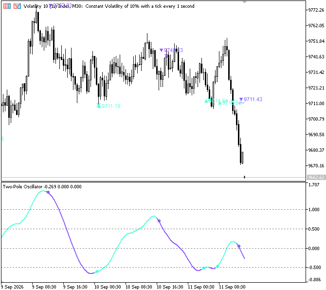
Figure 1. What We Are Building

Implementation Plan

Before we begin the implementation, let's explore the sequence of steps involved in building the Two-Pole Momentum Oscillator in MQL5.

1. Setting up the Indicator Properties and Buffers

Before calculating the oscillator values, we first need to define the basic structure of the indicator and prepare the buffers that will store the oscillator data, color information, and buy and sell signals. The implementation begins by defining the indicator framework, including its separate-window display, the number of buffers, the graphical plots, and the reference levels used to interpret the oscillator.

During this step, we will:

• define the indicator properties, including the separate-window display mode, four indicator buffers, and three graphical plots for the oscillator line, buy markers, and sell markers;
• configure the oscillator as a color-changing line using DRAW_COLOR_LINE, with separate colors representing its directional movement;
• configure the buy and sell plots as arrow markers that will be placed when momentum-shift conditions are detected;
• define horizontal reference levels at 1.0, 0.5, 0.0, -0.5, and -1.0 to provide a visual scale for interpreting the oscillator;
• create the four buffers used by the indicator, separating the oscillator values, color indexes, and buy and sell signal values;
• connect each buffer to its corresponding plot using SetIndexBuffer() and configure the buffers as non-series arrays so their indexes progress from older to newer bars.

This establishes the foundation for the indicator before we begin calculating the price deviation, normalization, and two-pole smoothing that produce the oscillator values.

2. Configuring Inputs, Plot Settings, and Calculation Structure

After setting up the indicator structure and buffers, we configure the input parameters, plot settings, and calculation structure that control how the Two-Pole Momentum Oscillator operates.

This includes:

• input parameters that allow users to adjust the filter length, level visibility, oscillator colors, and the number of historical bars used for drawing objects;
• plot settings that configure the color palette of the oscillator and the appearance of the buy and sell markers;
• empty-value settings that prevent unused buy and sell signal positions from being displayed on the indicator;
• a minimum historical data check that ensures enough bars are available before the oscillator calculations begin;
• recalculation logic that determines where processing should start during the initial calculation and subsequent indicator updates;
• a calculation loop that provides the structure for processing each available bar and performing the oscillator calculations.

3. Calculating Price Deviation from the Moving Average

At this stage, we begin measuring how far the current closing price has moved away from its recent average. The indicator uses a 25-period Simple Moving Average as the reference point. For every bar where enough historical data is available, the function calculates a 25-period moving average using the current bar and the previous 24 bars, then compares the current close with that average.

The indicator performs this calculation over 25 periods, but a smaller three-period example will make the process easier to visualize. The calculation remains the same, allowing us to understand the method without working through a larger set of candles.

Our 6 candles:

Bar	Open	High	Low	Close
Day 1	99.30	99.60	99.00	99.20
Day 2	99.20	99.40	98.80	99.00
Day 3	99.00	99.20	98.50	98.70
Day 4	98.70	99.10	98.60	98.90
Day 5	98.90	99.50	98.80	99.30
Day 6	99.30	100.00	99.10	99.80

Because our example uses a 3-period moving average, we cannot calculate the first two days. We need three closing prices before we can calculate the first average.

Average of Day 1, Day 2, and Day 3 closes:

 (99.20 + 99.00 + 98.70) ÷ 3 = 296.90 ÷ 3 = 98.9667

We then compare Day 3's closing price with this average:

 Drift = 98.70 − 98.9667 = −0.2667

The negative result means that Day 3 closed below its recent average.

Average of Day 2, Day 3, and Day 4:

(99.00 + 98.70 + 98.90) ÷ 3 = 296.60 ÷ 3 = 98.8667

Drift = 98.90 − 98.8667 = +0.0333

This time, the closing price is slightly above its recent average, so the deviation is positive.

Average of Day 3, Day 4, and Day 5:

(98.70 + 98.90 + 99.30) ÷ 3 = 296.90 ÷ 3 = 98.9667

Drift = 99.30 − 98.9667 = +0.3333

The positive value is larger because the closing price has moved farther above its recent average.

Average of Day 4, Day 5, and Day 6:

(98.90 + 99.30 + 99.80) ÷ 3 = 298.00 ÷ 3 = 99.3333

Drift = 99.80 − 99.3333 = +0.4667

Again, the closing price is above its recent average, and the larger positive deviation shows that the price is further above that average.

The result of this process is a new series containing the deviation of price from its moving average:

Bar	Price Deviation
Day 3	−0.2667
Day 4	+0.0333
Day 5	+0.3333
Day 6	+0.4667

In the actual implementation, we will use a 25-period moving average rather than the three-period average used in our simplified example. We will also provide a dynamic array to store the resulting price deviation values so they can be used in the next stages of the oscillator calculation.

This deviation series is important because it removes the absolute price level from the next stages of the calculation. Instead of working directly with prices such as 99.80 or 3,000, we now have values that describe the position of price relative to its own recent average. A positive value indicates that the price is above the average, while a negative value indicates that the price is below it.

4. Normalizing Price Deviation and Measuring Candle Range

The previous step gave us a series of deviation values showing how far each closing price was from its recent average. We now analyze this series to understand the current deviation in the context of its recent history. This helps us determine whether the current value represents a typical deviation or a relatively strong one.

To normalize these deviation values, we first calculate their average. We then measure their standard deviation to determine how much the values typically vary around that average. This gives us both the typical level of deviation and its usual amount of variation. We can continue with the simplified example from the previous step. Our available deviation history was:

Bar	Price Deviation
Day 3	−0.2667
Day 4	+0.0333
Day 5	+0.3333
Day 6	+0.4667

First, we calculate their average:

(−0.2667 + 0.0333 + 0.3333 + 0.4667) ÷ 4 = 0.14165

This tells us that the average deviation over these observations is approximately 0.1417. 

We then measure how far each deviation is from this average. For example, Day 6 has a deviation of 0.4667, so its difference from the average is:

0.4667 − 0.1417 = 0.3250

We square each deviation from the mean and sum the squared differences. We then divide by the number of observations and take the square root. The population standard deviation for our simplified example is roughly 0.2832, indicating the typical degree of variance around the average deviation. After that, we can normalize the current deviation using these two metrics. Day 6's current deviation is 0.4667, while the standard deviation is roughly 0.2832 and the recent average is at 0.1417. The normalized deviation using these numbers is:

(0.4667 − 0.1417) ÷ 0.2832 = 1.1475

A normalized deviation of 1.1475 means the current price deviation is about 1.1475 standard deviations above its recent average. This puts the current deviation into context by showing how it compares with its typical recent behavior. The actual indicator performs this normalization over a 25-period window and stores the resulting values for the next stage, where they are smoothed through two consecutive filtering stages. Each candle's range is calculated as high minus low. A 100-period average of these ranges estimates typical recent candle size. The normalized deviation will drive the oscillator, while the average candle range will later determine the dynamic price levels associated with its signals.

5. Applying Two-Pole Smoothing and Detecting Oscillator Direction

Overview: Normalized deviation values can change sharply from one bar to another. Smoothing reduces these rapid changes and turns the normalized values into a more stable oscillator line that is easier to interpret.

For this demonstration, we will use a Filter Length of 3 instead of the actual default of 15. This smaller value makes the calculation easier to follow manually.

Filter Length = 3

The smoothing factor is calculated as:

alpha = 2 ÷ (Filter Length + 1) = 0.5

First pass (smooth1): 

[(1−alpha) × Previous First Smoothed Value] + [alpha × Current Normalized Deviation]

The first smoothing stage takes the current normalized deviation and combines it with the previous value produced by the same smoothing stage. The first available normalized value is used to initialize the process.

For this smoothing demonstration, we will use the following normalized deviation values as hypothetical inputs. These values are provided only to demonstrate how the two smoothing stages work and are not being recalculated from the Day 3 to Day 6 deviation values above.

Using these illustrative normalized values:

• Day 3: There is no previous smoothed value yet, so the first value is used directly → −1.4420
• Day 4: 0.5 × (−1.4420) + 0.5 × (−0.3827) = −0.7210 + (−0.1914) = −0.9124
• Day 5: 0.5 × (−0.9124) + 0.5 × 0.6765 = −0.4562 + 0.3383 = −0.1179
• Day 6: 0.5 × (−0.1179) + 0.5 × 1.1475 = −0.0590 + 0.5738 = +0.5148

The first pass has already reduced the sharp movement in the normalized values. Instead of moving directly from −0.3827 to +0.6765 and then +1.1475, the smoothed values move more gradually.

Second pass (smooth2): 

[(1−alpha) × Previous Second Smoothed Value] + [alpha × Current First Smoothed Value]

The second smoothing stage applies the same process again, but this time it does not use the original normalized deviation. It uses the values produced by the first smoothing stage. This gives the oscillator another layer of smoothing.

• Day 3: The process starts with the first smoothed value → −1.4420
• Day 4: 0.5 × (−1.4420) + 0.5 × (−0.9124) = −0.7210 + (−0.4562) = −1.1772
• Day 5: 0.5 × (−1.1772) + 0.5 × (−0.1179) = −0.5886 + (−0.0590) = −0.6476
• Day 6: 0.5 × (−0.6476) + 0.5 × 0.5148 = −0.3238 + 0.2574 = −0.0664

The second pass produces an even smoother series because it is smoothing the already-smoothed values from the first pass. This second smoothing result becomes the actual oscillator line displayed by the indicator.

The result carried into the next stage is therefore:

Bar	Line value
Day 3	−1.4420
Day 4	−1.1772
Day 5	−0.6476
Day 6	−0.0664

This gives us the final Two-Pole oscillator values, which we can now compare with their values four bars earlier to determine whether the oscillator has moved upward or downward.

6. Turning Oscillator Signals into Dynamic Control Levels

At this stage, the indicator moves from calculating oscillator values to displaying and managing signals on the price chart. It compares the current oscillator value with its value four bars earlier to determine its movement over that interval. A buy condition occurs when the current value is higher than the earlier value while remaining below zero, whereas a sell condition occurs when the current value is lower than the earlier value while remaining above zero. Since this comparison requires historical data, a safe fallback is used when there are not yet enough bars. Once a signal is confirmed, the indicator calculates a dynamic control level using the signal candle's low or high and the previously calculated average candle range. It then creates an active control line and a price marker with unique names so they can be managed later.

Only one direction can remain active at a time, so a new buy condition removes an active sell control line, and vice versa. The triangle and price marker from the previous condition remain on the chart as historical markers. The indicator continues monitoring the active control level and places an X marker when price crosses it, then removes the active control line and deactivates that level. Chart objects are managed only for closed candles and within the selected display range, preventing incomplete candle data from being used to create or update these objects. If a control level remains active, its line is extended to the latest bar. Overall, this step implements buy/sell condition detection, dynamic control-level creation, and chart-object management.

Implementation in MQL5

Following the previously defined implementation plan, we will now create the Two-Pole Momentum Oscillator in MQL5 by developing each required function, calculation process, signal condition, and chart-display element individually.

Setting up the Indicator Properties and Buffers

First, set up the indicator properties and buffers.

Example:

#property indicator_separate_window
#property indicator_buffers 4
#property indicator_plots   3

//--- oscillator line (color index 0=neutral, 1=up, 2=down)
#property indicator_type1   DRAW_COLOR_LINE
#property indicator_color1  clrSilver, clrAqua, clrPurple
#property indicator_width1  2
#property indicator_label1  "Two-Pole"

//--- buy markers
#property indicator_type2   DRAW_ARROW
#property indicator_color2  clrAqua
#property indicator_width2  2
#property indicator_label2  "Buy"

//--- sell markers
#property indicator_type3   DRAW_ARROW
#property indicator_color3  clrPurple
#property indicator_width3  2
#property indicator_label3  "Sell"

//--- reference gridlines
#property indicator_level1     1.0
#property indicator_level2     0.5
#property indicator_level3     0.0
#property indicator_level4    -0.5
#property indicator_level5    -1.0
#property indicator_levelcolor clrGray
#property indicator_levelstyle STYLE_DOT
#property indicator_levelwidth 1

#define OBJ_PREFIX "TPO_"

//-- buffers
double Two_p[];        // the final, double-smoothed oscillator value for each bar (what gets plotted as the line)
double Two_pColor[];   // color index per bar for Two_p: 0=neutral, 1=up color, 2=down color
double BuyArrow[];     // holds Two_p[i] on bars where a buy signal fired, EMPTY_VALUE everywhere else
double SellArrow[];    // holds Two_p[i] on bars where a sell signal fired, EMPTY_VALUE everywhere else

//+------------------------------------------------------------------+
//| Custom indicator initialization function                         |
//+------------------------------------------------------------------+
int OnInit()
  {
//--- bind each array to its buffer slot; order here must match the #property plot declarations above
   SetIndexBuffer(0, Two_p,      INDICATOR_DATA);
   SetIndexBuffer(1, Two_pColor, INDICATOR_COLOR_INDEX);   // color index buffer paired with buffer 0's DRAW_COLOR_LINE
   SetIndexBuffer(2, BuyArrow,   INDICATOR_DATA);
   SetIndexBuffer(3, SellArrow,  INDICATOR_DATA);

//--- we calculate chronologically (oldest bar first), so all buffers are treated as non-series arrays
   ArraySetAsSeries(Two_p,      false);
   ArraySetAsSeries(Two_pColor, false);
   ArraySetAsSeries(BuyArrow,   false);
   ArraySetAsSeries(SellArrow,  false);

   IndicatorSetString(INDICATOR_SHORTNAME, "Two-Pole Oscillator");

//---
   return(INIT_SUCCEEDED);
  }
//+------------------------------------------------------------------+
//| Custom indicator iteration function                              |
//+------------------------------------------------------------------+
int OnCalculate(const int32_t rates_total,
                const int32_t prev_calculated,
                const datetime &time[],
                const double &open[],
                const double &high[],
                const double &low[],
                const double &close[],
                const long &tick_volume[],
                const long &volume[],
                const int32_t &spread[])
  {
//---

//--- return value of prev_calculated for next call
   return(rates_total);
  }
//+------------------------------------------------------------------+

Explanation:

The first part establishes the indicator's structure by placing the Two-Pole oscillator in a separate subwindow, allocating four buffers for the oscillator values, color indexes, and buy and sell markers, and defining three visual plots. The plot settings determine how the oscillator changes color and how the signal markers appear, while horizontal levels at 1.0, 0.5, 0.0, -0.5, and -1.0 provide reference points for interpreting oscillator values. A common TPO_ prefix identifies the chart objects created by the indicator, making them easier to manage and remove. During initialization, OnInit() connects the buffers to their respective plots and configures chronological processing, ensuring that calculated values and visual elements are handled consistently.

Configuring Inputs, Plot Settings, and Calculation Structure

Next, set up the indicator inputs and calculation parameters.

Example:

#define OBJ_PREFIX "TPO_"

//-- buffers
double Two_p[];                           // the final, double-smoothed oscillator value for each bar (what gets plotted as the line)
double Two_pColor[];                      // color index per bar for Two_p: 0=neutral, 1=up color, 2=down color
double BuyArrow[];                        // holds Two_p[i] on bars where a buy signal fired, EMPTY_VALUE everywhere else
double SellArrow[];                       // holds Two_p[i] on bars where a sell signal fired, EMPTY_VALUE everywhere else

//--- inputs
input int   InpLength      = 15;              // Filter Length
input bool  InpShowLevels  = true;            // Show dynamic control lines
input color InpUpColor     = C'85,255,218';   // Up color
input color InpDnColor     = C'140,91,255';   // Down color
input int   InpDisplayBars = 500;             // Bars back to draw objects on (0 = all)

//+------------------------------------------------------------------+
//| Custom indicator initialization function                         |
//+------------------------------------------------------------------+
int OnInit()
  {
//--- bind each array to its buffer slot; order here must match the #property plot declarations above
   SetIndexBuffer(0, Two_p,      INDICATOR_DATA);
   SetIndexBuffer(1, Two_pColor, INDICATOR_COLOR_INDEX);   // color index buffer paired with buffer 0's DRAW_COLOR_LINE
   SetIndexBuffer(2, BuyArrow,   INDICATOR_DATA);
   SetIndexBuffer(3, SellArrow,  INDICATOR_DATA);

//--- we calculate chronologically (oldest bar first), so all buffers are treated as non-series arrays
   ArraySetAsSeries(Two_p,      false);
   ArraySetAsSeries(Two_pColor, false);
   ArraySetAsSeries(BuyArrow,   false);
   ArraySetAsSeries(SellArrow,  false);

   IndicatorSetString(INDICATOR_SHORTNAME, "Two-Pole Oscillator");

//--- apply the user's chosen colors to the line's 3 color-index slots (0=neutral, 1=up, 2=down)
   PlotIndexSetInteger(0, PLOT_LINE_COLOR, 0, clrSilver);
   PlotIndexSetInteger(0, PLOT_LINE_COLOR, 1, InpUpColor);
   PlotIndexSetInteger(0, PLOT_LINE_COLOR, 2, InpDnColor);

//--- buy arrow plot: small circle (Wingdings code 159), colored with the user's up color
   PlotIndexSetInteger(1, PLOT_ARROW, 159);
   PlotIndexSetInteger(1, PLOT_LINE_COLOR, InpUpColor);
   PlotIndexSetDouble(1, PLOT_EMPTY_VALUE, EMPTY_VALUE);   // bars without a signal are skipped, not drawn as 0

//--- sell arrow plot: same marker shape, colored with the user's down color
   PlotIndexSetInteger(2, PLOT_ARROW, 159);
   PlotIndexSetInteger(2, PLOT_LINE_COLOR, InpDnColor);
   PlotIndexSetDouble(2, PLOT_EMPTY_VALUE, EMPTY_VALUE);

//--- validate filter length
   if(InpLength < 1)
     {
      Print("InpLength must be greater than 0.");
      return(INIT_PARAMETERS_INCORRECT);
     }

//---
   return(INIT_SUCCEEDED);
  }
//+------------------------------------------------------------------+
//| Custom indicator iteration function                              |
//+------------------------------------------------------------------+
int OnCalculate(const int32_t rates_total,
                const int32_t prev_calculated,
                const datetime &time[],
                const double &open[],
                const double &high[],
                const double &low[],
                const double &close[],
                const long &tick_volume[],
                const long &volume[],
                const int32_t &spread[])
  {
//---
   if(rates_total < 130)   // not enough bars yet for the longest lookback (100) plus warm-up room; bail out safely
      return(0);

//--- work chronologically, oldest bar at index 0, so our recursive filter and lookback math read naturally
   ArraySetAsSeries(time,  false);
   ArraySetAsSeries(high,  false);
   ArraySetAsSeries(low,   false);
   ArraySetAsSeries(close, false);

//--- only recompute what's new: on a normal tick, start one bar back from where we left off (that bar may have
//--- changed from an unfinished candle into a finished one); on the very first run, start from the beginning
   int start = (prev_calculated > 1) ? prev_calculated-1 : 0;

   for(int i = start; i < rates_total; i++)
     {

     }

//--- return value of prev_calculated for next call
   return(rates_total);
  }
//+------------------------------------------------------------------+

Explanation:

The input section allows users to customize the indicator's behavior and appearance. InpLength sets the filter length, with a default value of 15, while InpShowLevels controls whether dynamic control lines are displayed. The InpUpColor and InpDnColor inputs define the colors used to represent upward and downward oscillator movements. Meanwhile, InpDisplayBars limits the historical range in which chart objects can be drawn, using 500 bars by default, while a value of 0 allows objects to be displayed across all available bars. During initialization, these settings are applied to the oscillator and signal plots. The oscillator uses three color indexes to represent its displayed states, while the buy and sell plots use small circle markers that remain hidden when no corresponding signal value is available.

Before processing begins, the indicator validates InpLength to prevent an invalid filter length from being used. It also requires at least 130 available bars, providing sufficient history for the longest lookback period and the additional initialization needed by the calculations. Price and time arrays are configured for chronological processing, with the oldest bar at index 0 and the newest at the highest index. The calculation then selects a starting position based on whether the indicator is running for the first time or updating previously calculated data. During an update, processing begins one bar before the previous calculation endpoint so that the most recently calculated bar can be refreshed if necessary. On the initial run, processing starts from the first available bar. From that point, the indicator works through the remaining bars to update its calculated values and associated signals.

Calculating Price Deviation from the Moving Average

Next, calculate how far the current price is from its moving average to measure its deviation from the average recent level.

Example:

//--- persistent working arrays (recursive filter needs history across ticks)
double g_diff[];      // close - sma1

//+--------------------------------------------------------------------+
//| Simple moving average over the window [i-period+1 .. i]            |
//| src[] must be a non-series array (index 0 = oldest bar)            |
//+--------------------------------------------------------------------+
double SMA_range(const double &src[], int i, int period)
  {
   if(i < period-1)                       // not enough bars behind us yet to fill a full window -> treat as "not available"
      return(0.0);
   double sum = 0.0;
   for(int k = i-period+1; k <= i; k++)   // walk every bar in the lookback window, oldest to newest
      sum += src[k];
   return(sum/period);                    // arithmetic mean of the window
  }

//+------------------------------------------------------------------+
//| Custom indicator iteration function                              |
//+------------------------------------------------------------------+
int OnCalculate(const int32_t rates_total,
                const int32_t prev_calculated,
                const datetime &time[],
                const double &open[],
                const double &high[],
                const double &low[],
                const double &close[],
                const long &tick_volume[],
                const long &volume[],
                const int32_t &spread[])
  {
//---
   if(rates_total < 130)   // not enough bars yet for the longest lookback (100) plus warm-up room; bail out safely
      return(0);

//--- work chronologically, oldest bar at index 0, so our recursive filter and lookback math read naturally
   ArraySetAsSeries(time,  false);
   ArraySetAsSeries(high,  false);
   ArraySetAsSeries(low,   false);
   ArraySetAsSeries(close, false);

//--- grow the persistent working arrays to match the current chart size (cheap no-op if already the right size)
   ArrayResize(g_diff, rates_total);

//--- only recompute what's new: on a normal tick, start one bar back from where we left off (that bar may have
//--- changed from an unfinished candle into a finished one); on the very first run, start from the beginning
   int start = (prev_calculated > 1) ? prev_calculated-1 : 0;

   for(int i = start; i < rates_total; i++)
     {
      //--- first valid 25-bar average is at index 24
      if(i < 24)
         continue;

      //--- how far is this bar's close from its own 25-bar moving average?
      double sma1 = SMA_range(close, i, 25);
      g_diff[i]   = close[i]-sma1;
     }

//--- return value of prev_calculated for next call
   return(rates_total);
  }
//+------------------------------------------------------------------+

Explanation:

The SMA_range() function calculates a Simple Moving Average from the specified source array over a given lookback period. It first checks whether enough bars are available to form a complete window, returning zero when the required data is insufficient. Otherwise, it adds the values within the window and divides their sum by the period to obtain the average. Since the window includes the current bar and the preceding bars, the result represents the average across the specified number of bars ending at the current position.

In the main calculation, g_diff is resized to accommodate the available chart history, and the starting position determines which bars need to be recalculated. Processing skips bars before index 24 because a complete 25-bar window is not available until that point. For each eligible bar, the indicator calculates the 25-period SMA of the closing prices and subtracts it from the current close. This difference is stored in g_diff[i], forming a series that measures how far the closing price lies above or below its recent average. Rather than using the raw closing price directly, the indicator uses this deviation series as the basis for the subsequent normalization and smoothing stages.

Normalizing Price Deviation and Measuring Candle Range

Next, normalize the price deviation to measure its strength relative to recent volatility while also calculating the average candle range for dynamic price targets.

Example:

//+--------------------------------------------------------------------+
//| Population standard deviation over the same [i-period+1 .. i]      |
//| window. Divides by 'period' (not period-1), matching a population  |
//| standard deviation rather than a sample standard deviation.        |
//+--------------------------------------------------------------------+
double StDev_range(const double &src[], int i, int period)
  {
   if(i < period-1)              // same warm-up guard as SMA_range
      return(0.0);
   double mean = SMA_range(src, i, period);   // step 1: average of the window
   double sumsq = 0.0;
   for(int k = i-period+1; k <= i; k++)
     {
      double d = src[k]-mean;    // step 2: how far this bar's value is from the average
      sumsq += d*d;              // step 3: square it (removes sign, weights bigger deviations more) and accumulate
     }
   return(MathSqrt(sumsq/period));   // step 4: average the squared deviations, step 5: square root -> std dev
  }

ArrayResize(g_diff, rates_total);
ArrayResize(g_range,    rates_total);

//--- only recompute what's new: on a normal tick, start one bar back from where we left off (that bar may have
//--- changed from an unfinished candle into a finished one); on the very first run, start from the beginning
int start = (prev_calculated > 1) ? prev_calculated-1 : 0;

for(int i = start; i < rates_total; i++)
  {
//--- "typical candle size" over the last 100 bars
   g_range[i]  = high[i]-low[i];

//--- first valid 25-bar average is at index 24
   if(i < 24)
      continue;

//--- how far is this bar's close from its own 25-bar moving average?
   double sma1 = SMA_range(close, i, 25);
   g_diff[i]   = close[i]-sma1;

//--- first bar where the 25-bar window of g_diff holds only real values
   if(i < 48)
      continue;

//--- standardize that drift into a z-score relative to its recent distribution
   double smaDiff   = SMA_range(g_diff, i, 25);
   double stdevDiff = StDev_range(g_diff, i, 25);
   double sma_n1    = (stdevDiff != 0.0) ? (g_diff[i]-smaDiff)/stdevDiff : 0.0;

//--- first valid 100-bar average of candle range is at index 99
   if(i < 99)
      continue;

   double area = SMA_range(g_range, i, 100);
  }
//+------------------------------------------------------------------+

Explanation:

To measure the spread of the deviation values, the StDev_range() function calculates the standard deviation over the same lookback period used for the moving average. The standard deviation is obtained by first confirming that a full window of data is available, then calculating the average of those values, squaring and adding up each value's deviation from the average, dividing the total by the number of observations, and taking the square root of this result.

In the main calculation, the range array is resized to match the number of available bars. Because the first valid `g_diff` value occurs at index 24, the calculation skips bars before index 48 so that the 25-bar window used for the standard deviation and average of `g_diff` contains only valid deviation values. The 25-period average and standard deviation of the price deviation values are then used to convert the current deviation into a z-score, allowing the current deviation to be compared with its recent behavior. At the same time, each candle's range is calculated from its high and low prices and stored for later use. Because a 100-period average requires 100 candle ranges, the calculation skips bars before index 99, making index 99 the first bar with a complete 100-bar range window. This average is then used to determine how far the dynamic control levels should be placed from the candle where the condition occurs.

Applying Two-Pole Smoothing and Detecting Oscillator Direction

Next, smooth the normalized deviation twice to produce a cleaner oscillator and compare its current value with its value four bars earlier to identify upward or downward movement.

Example:

//--- persistent working arrays (recursive filter needs history across ticks)
double g_diff[];      // close - sma1
double g_range[];     // high - low
double g_smooth1[];
double g_smooth2[];

//--- grow the persistent working arrays to match the current chart size (cheap no-op if already the right size)
ArrayResize(g_diff, rates_total);
ArrayResize(g_range,    rates_total);
ArrayResize(g_smooth1,  rates_total);
ArrayResize(g_smooth2,  rates_total);

//--- only recompute what's new: on a normal tick, start one bar back from where we left off (that bar may have
//--- changed from an unfinished candle into a finished one); on the very first run, start from the beginning
int start = (prev_calculated > 1) ? prev_calculated-1 : 0;

double alpha = 2.0/(InpLength+1);   // convert the user's "Filter Length" input into an EMA-style smoothing weight

for(int i = start; i < rates_total; i++)
  {
//--- default every bar to "nothing to draw"; valid bars overwrite these below
   Two_p[i]      = EMPTY_VALUE;
   Two_pColor[i] = 0;

//--- "typical candle size" over the last 100 bars
   g_range[i]  = high[i]-low[i];

//--- first valid 25-bar average is at index 24
   if(i < 24)
      continue;

//--- how far is this bar's close from its own 25-bar moving average?
   double sma1 = SMA_range(close, i, 25);
   g_diff[i]   = close[i]-sma1;

//--- first bar where the 25-bar window of g_diff holds only real values
   if(i < 48)
      continue;

//--- standardize that drift into a z-score relative to its recent distribution
   double smaDiff   = SMA_range(g_diff, i, 25);
   double stdevDiff = StDev_range(g_diff, i, 25);
   double sma_n1    = (stdevDiff != 0.0) ? (g_diff[i]-smaDiff)/stdevDiff : 0.0;

//--- standardize that drift into a z-score, so the reading is comparable across any instrument
   if(i < 99)
      continue;

   double area = SMA_range(g_range, i, 100);

//--- two-pole filter - two EMA-style smoothing passes chained together
   if(i == 99 )
     {
      //--- no prior bar exists yet, so seed both stages directly with today's raw value instead of blending
      g_smooth1[i] = sma_n1;
      g_smooth2[i] = sma_n1;
     }
   else
     {
      //--- first pass: blend yesterday's smooth1 with today's fresh z-score
      g_smooth1[i] = (1-alpha)*g_smooth1[i-1] + alpha*sma_n1;
      //--- second pass: blend yesterday's smooth2 with today's just-computed smooth1 (smooths the smoothed line)
      g_smooth2[i] = (1-alpha)*g_smooth2[i-1] + alpha*g_smooth1[i];
     }

   Two_p[i] = g_smooth2[i];   // this is the final oscillator value plotted on the chart

//--- reference point for detecting a turn = this same line's value 4 bars ago
   double two_pp = (i >= 4) ? Two_p[i-4] : Two_p[i];   // fall back to today's own value if 4 bars back doesn't exist yet

//--- color the line by direction: above its own reference = "up" color, at/below = "down" color
   Two_pColor[i] = (Two_p[i] > two_pp) ? 1 : 2;

  }

Output:

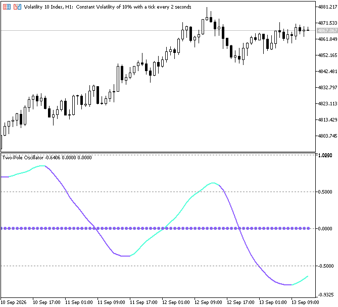
Figure 2. First and Second Smoothing

Explanation:

The two-pole filter applies two consecutive EMA-style smoothing stages to the normalized deviation. On the first bar, both stages are initialized with the raw normalized value because there is no previous value available for the calculation. From the following bars onward, the first stage smooths the current normalized deviation using the previous smoothed value, while the second stage applies another smoothing pass to the result from the first stage. This produces a smoother oscillator value with less short-term fluctuation. The final value from the second stage is stored in Two_p[i], which is the main indicator buffer responsible for plotting the Two-Pole oscillator.

Next, the indicator looks four bars back to create a reference value. When four bars of history are not yet available, the current Two_p value is used as the fallback reference. The current Two_p value is then compared with this reference, and the indicator stores color index 1 for an upward-moving oscillator or color index 2 otherwise in Two_pColor, which is the color-index buffer used to control the color of the oscillator line.

Turning Oscillator Signals into Dynamic Control Levels

Next, convert valid oscillator conditions into dynamic control levels and manage their chart objects.

Example:

//--- state for the single active buy/sell target line. Only one of each can be "live" at a time -
//--- a new opposite signal cancels whichever one is currently active.
string g_buyLineName  = "";
string g_sellLineName = "";
bool   g_buyActive     = false;
bool   g_sellActive    = false;
double g_buyLevel      = 0.0;   // price level of the currently active buy target line
double g_sellLevel     = 0.0;   // price level of the currently active sell target line

//+------------------------------------------------------------------+
//| Create / update / retire the target-line and label objects       |
//| Called only for closed bars that fall inside the display window  |
//+------------------------------------------------------------------+
void ManageObjects(bool buy, bool sell, int i, const datetime &time[],
                   const double &low[], const double &high[], double area)
  {
//--- new buy signal: cancel any active sell line, start a fresh buy line + tags
   if(buy)
     {
      if(g_sellActive)
        {
         ResetLastError();
         if(ObjectDelete(0, g_sellLineName))
            g_sellActive = false;
         else
            Print("Failed to delete sell line: ", g_sellLineName,
                  ". Error: ", GetLastError());
        }

      double level = low[i]-area;
      g_buyLevel    = level;
      g_buyActive   = true;
      g_buyLineName = OBJ_PREFIX+"BuyLine_"+IntegerToString((int)time[i]);

      if(InpShowLevels)
        {
         ResetLastError();
         if(ObjectCreate(0, g_buyLineName, OBJ_TREND, 0, time[i], level, time[i], level))
           {
            ObjectSetInteger(0, g_buyLineName, OBJPROP_COLOR, InpUpColor);
            ObjectSetInteger(0, g_buyLineName, OBJPROP_STYLE, STYLE_DASH);
            ObjectSetInteger(0, g_buyLineName, OBJPROP_WIDTH, 1);
            ObjectSetInteger(0, g_buyLineName, OBJPROP_RAY_RIGHT, false);
           }
         else
            Print("Failed to create buy line: ", g_buyLineName,
                  ". Error: ", GetLastError());
        }

      string tagName = OBJ_PREFIX+"BuyTag_"+IntegerToString((int)time[i]);
      ResetLastError();
      if(ObjectCreate(0, tagName, OBJ_TEXT, 0, time[i], level))
        {
         ObjectSetString(0, tagName, OBJPROP_TEXT, "\x25B2 "+DoubleToString(level, _Digits));
         ObjectSetInteger(0, tagName, OBJPROP_COLOR, InpUpColor);
         ObjectSetInteger(0, tagName, OBJPROP_ANCHOR, ANCHOR_LEFT_UPPER);
         ObjectSetInteger(0, tagName, OBJPROP_FONTSIZE, 8);
        }
      else
         Print("Failed to create buy tag: ", tagName,
               ". Error: ", GetLastError());
     }

//--- new sell signal: cancel any active buy line, start a fresh sell line + tags
   if(sell)
     {
      if(g_buyActive)
        {
         ResetLastError();
         if(ObjectDelete(0, g_buyLineName))
            g_buyActive = false;
         else
            Print("Failed to delete buy line: ", g_buyLineName,
                  ". Error: ", GetLastError());
        }

      double level = high[i]+area;
      g_sellLevel    = level;
      g_sellActive   = true;
      g_sellLineName = OBJ_PREFIX+"SellLine_"+IntegerToString((int)time[i]);

      if(InpShowLevels)
        {
         ResetLastError();
         if(ObjectCreate(0, g_sellLineName, OBJ_TREND, 0, time[i], level, time[i], level))
           {
            ObjectSetInteger(0, g_sellLineName, OBJPROP_COLOR, InpDnColor);
            ObjectSetInteger(0, g_sellLineName, OBJPROP_STYLE, STYLE_DASH);
            ObjectSetInteger(0, g_sellLineName, OBJPROP_WIDTH, 1);
            ObjectSetInteger(0, g_sellLineName, OBJPROP_RAY_RIGHT, false);
           }
         else
            Print("Failed to create sell line: ", g_sellLineName,
                  ". Error: ", GetLastError());
        }

      string tagName = OBJ_PREFIX+"SellTag_"+IntegerToString((int)time[i]);
      ResetLastError();
      if(ObjectCreate(0, tagName, OBJ_TEXT, 0, time[i], level))
        {
         ObjectSetString(0, tagName, OBJPROP_TEXT, "\x25BC "+DoubleToString(level, _Digits));
         ObjectSetInteger(0, tagName, OBJPROP_COLOR, InpDnColor);
         ObjectSetInteger(0, tagName, OBJPROP_ANCHOR, ANCHOR_LEFT_LOWER);
         ObjectSetInteger(0, tagName, OBJPROP_FONTSIZE, 8);
        }
      else
         Print("Failed to create sell tag: ", tagName,
               ". Error: ", GetLastError());
     }

//--- price later trades back down through an active buy level -> stamp X, retire the line
   if(!buy && g_buyActive && i >= 1 && low[i-1] >= g_buyLevel && low[i] < g_buyLevel)
     {
      string xName = OBJ_PREFIX+"BuyX_"+IntegerToString((int)time[i]);
      ResetLastError();
      if(ObjectCreate(0, xName, OBJ_TEXT, 0, time[i], g_buyLevel))
        {
         ObjectSetString(0, xName, OBJPROP_TEXT, "\x2716");
         ObjectSetInteger(0, xName, OBJPROP_COLOR, InpUpColor);
         ObjectSetInteger(0, xName, OBJPROP_ANCHOR, ANCHOR_CENTER);
         ObjectSetInteger(0, xName, OBJPROP_FONTSIZE, 10);
        }
      else
         Print("Failed to create buy X marker: ", xName,
               ". Error: ", GetLastError());

      ResetLastError();
      if(ObjectDelete(0, g_buyLineName))
         g_buyActive = false;
      else
         Print("Failed to delete buy line: ", g_buyLineName,
               ". Error: ", GetLastError());
     }

//--- price later trades back up through an active sell level -> stamp X, retire the line
   if(!sell && g_sellActive && i >= 1 && high[i-1] <= g_sellLevel && high[i] > g_sellLevel)
     {
      string xName = OBJ_PREFIX+"SellX_"+IntegerToString((int)time[i]);
      ResetLastError();
      if(ObjectCreate(0, xName, OBJ_TEXT, 0, time[i], g_sellLevel))
        {
         ObjectSetString(0, xName, OBJPROP_TEXT, "\x2716");
         ObjectSetInteger(0, xName, OBJPROP_COLOR, InpDnColor);
         ObjectSetInteger(0, xName, OBJPROP_ANCHOR, ANCHOR_CENTER);
         ObjectSetInteger(0, xName, OBJPROP_FONTSIZE, 10);
        }
      else
         Print("Failed to create sell X marker: ", xName,
               ". Error: ", GetLastError());

      ResetLastError();
      if(ObjectDelete(0, g_sellLineName))
         g_sellActive = false;
      else
         Print("Failed to delete sell line: ", g_sellLineName,
               ". Error: ", GetLastError());
     }
  }
//+------------------------------------------------------------------+

//+------------------------------------------------------------------+
//| Custom indicator Deinitialization function                       |
//+------------------------------------------------------------------+
void OnDeinit(const int reason)
  {
   if(reason == REASON_REMOVE)
     {
      ResetLastError();
      int deleted = ObjectsDeleteAll(0, OBJ_PREFIX, -1, -1);

      if(deleted < 0)
         Print("Failed to delete objects with prefix: ", OBJ_PREFIX,
               ". Error: ", GetLastError());
     }
  }
//+------------------------------------------------------------------+
//| Custom indicator iteration function                              |
//+------------------------------------------------------------------+
int OnCalculate(const int32_t rates_total,
                const int32_t prev_calculated,
                const datetime &time[],
                const double &open[],
                const double &high[],
                const double &low[],
                const double &close[],
                const long &tick_volume[],
                const long &volume[],
                const int32_t &spread[])
  {
//---
   if(rates_total < 130)   // not enough bars yet for the longest lookback (100) plus warm-up room; bail out safely
      return(0);

//--- work chronologically, oldest bar at index 0, so our recursive filter and lookback math read naturally
   ArraySetAsSeries(time,  false);
   ArraySetAsSeries(high,  false);
   ArraySetAsSeries(low,   false);
   ArraySetAsSeries(close, false);

//--- grow the persistent working arrays to match the current chart size (cheap no-op if already the right size)
   ArrayResize(g_diff, rates_total);
   ArrayResize(g_range,    rates_total);
   ArrayResize(g_smooth1,  rates_total);
   ArrayResize(g_smooth2,  rates_total);

//--- only recompute what's new: on a normal tick, start one bar back from where we left off (that bar may have
//--- changed from an unfinished candle into a finished one); on the very first run, start from the beginning
   int start = (prev_calculated > 1) ? prev_calculated-1 : 0;

//--- full recalculation: wipe old objects/state so we don't leave orphans behind
   if(prev_calculated == 0)
     {
      ObjectsDeleteAll(0, OBJ_PREFIX, -1, -1);
      g_buyActive = false;
      g_sellActive = false;
      g_buyLineName = "";
      g_sellLineName = "";
     }

   double alpha = 2.0/(InpLength+1);   // convert the user's "Filter Length" input into an EMA-style smoothing weight

   for(int i = start; i < rates_total; i++)
     {
      //--- default every bar to "nothing to draw"; valid bars overwrite these below
      Two_p[i]      = EMPTY_VALUE;
      Two_pColor[i] = 0;
      BuyArrow[i]   = EMPTY_VALUE;
      SellArrow[i]  = EMPTY_VALUE;

      //--- "typical candle size" over the last 100 bars
      g_range[i]  = high[i]-low[i];

      //--- first valid 25-bar average is at index 24
      if(i < 24)
         continue;

      //--- how far is this bar's close from its own 25-bar moving average?
      double sma1 = SMA_range(close, i, 25);
      g_diff[i]   = close[i]-sma1;

      //--- first bar where the 25-bar window of g_diff holds only real values
      if(i < 48)
         continue;

      //--- standardize that drift into a z-score relative to its recent distribution
      double smaDiff   = SMA_range(g_diff, i, 25);
      double stdevDiff = StDev_range(g_diff, i, 25);
      double sma_n1    = (stdevDiff != 0.0) ? (g_diff[i]-smaDiff)/stdevDiff : 0.0;

      //--- first valid 100-bar average of candle range is at index 99
      if(i < 99)
         continue;

      double area = SMA_range(g_range, i, 100);

      //--- two-pole filter - two EMA-style smoothing passes chained together
      if(i == 99 )
        {
         //--- no prior bar exists yet, so seed both stages directly with today's raw value instead of blending
         g_smooth1[i] = sma_n1;
         g_smooth2[i] = sma_n1;
        }
      else
        {
         //--- first pass: blend yesterday's smooth1 with today's fresh z-score
         g_smooth1[i] = (1-alpha)*g_smooth1[i-1] + alpha*sma_n1;
         //--- second pass: blend yesterday's smooth2 with today's just-computed smooth1 (smooths the smoothed line)
         g_smooth2[i] = (1-alpha)*g_smooth2[i-1] + alpha*g_smooth1[i];
        }

      Two_p[i] = g_smooth2[i];   // this is the final oscillator value plotted on the chart

      //--- reference point for detecting a turn = this same line's value 4 bars ago
      double two_pp = (i >= 4) ? Two_p[i-4] : Two_p[i];   // fall back to today's own value if 4 bars back doesn't exist yet

      //--- color the line by direction: above its own reference = "up" color, at/below = "down" color
      Two_pColor[i] = (Two_p[i] > two_pp) ? 1 : 2;

      //--- i >= 5 ensures both today's and yesterday's reference points (i-4 and i-5) are valid array indices
      if(i >= 5)
        {
         double prevTwoP  = Two_p[i-1];                                   // yesterday's line value
         double prevTwoPp = (i-1 >= 4) ? Two_p[i-5] : Two_p[i-1];         // yesterday's reference (4 bars before yesterday)

         //--- Step 5: a true crossover needs BOTH days' relationships - at/below yesterday, above today (for buy) -
         //--- plus the "still stretched" filter (line below zero for buy, above zero for sell)
         bool buy  = (prevTwoP <= prevTwoPp && Two_p[i] > two_pp && Two_p[i] < 0.0);
         bool sell = (prevTwoP >= prevTwoPp && Two_p[i] < two_pp && Two_p[i] > 0.0);

         if(buy)
            BuyArrow[i]  = Two_p[i];   // plot a marker at the oscillator's own value on this bar
         if(sell)
            SellArrow[i] = Two_p[i];

         //--- gate chart-object drawing separately from signal detection: signals above are calculated on every
         //--- bar regardless, but we only ever draw a line/label/X-mark when both of these are true
         bool closedBar     = (i < rates_total-1);                              // never draw on the still-forming bar
         bool withinDisplay = (InpDisplayBars <= 0) || (i >= rates_total-InpDisplayBars);   // inside the user's lookback window

         if(closedBar && withinDisplay)
            ManageObjects(buy, sell, i, time, low, high, area);
        }
     }

//--- extend any still-active lines out to the latest bar
   if(g_buyActive)
     {
      ResetLastError();
      if(!ObjectMove(0, g_buyLineName, 1, time[rates_total-1], g_buyLevel))
         Print("Failed to move buy line: ", g_buyLineName,
               ". Error: ", GetLastError());
     }

   if(g_sellActive)
     {
      ResetLastError();
      if(!ObjectMove(0, g_sellLineName, 1, time[rates_total-1], g_sellLevel))
         Print("Failed to move sell line: ", g_sellLineName,
               ". Error: ", GetLastError());
     }

//--- return value of prev_calculated for next call
   return(rates_total);
  }
//+------------------------------------------------------------------+

Output:

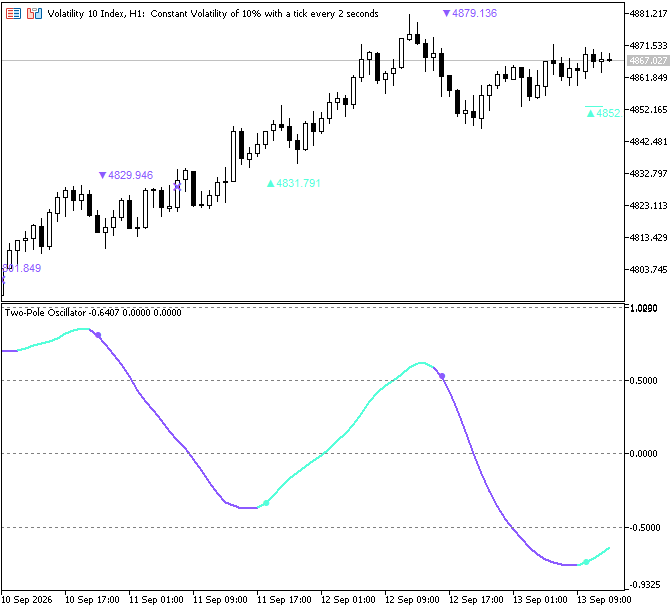
Figure 3. Two-Pole Oscillator

Explanation:

The ManageObjects() function manages the lifecycle of the dynamic control levels and their associated chart objects. It distinguishes the active control line from the historical markers: the line represents the current level being monitored, while the triangle and price label preserve the location of the original buy or sell condition. When a new buy condition occurs, any active sell control line is removed, and the buy control level is calculated below the condition candle using its low and the average candle range. The function stores the level, marks it as active, and creates the corresponding dashed line and upward price marker when control-line display is enabled. For a sell condition, the process is reversed, with the control level placed above the condition candle's high and the corresponding sell objects created.

While a control level remains active, the function monitors price for a crossing. A downward crossing of an active buy level or an upward crossing of an active sell level triggers an X marker at the crossed level. The corresponding control line is then deleted, and the level is marked as inactive. The original triangle and price label remain on the chart to preserve the historical signal, even after the active level has been deactivated.

During a full recalculation, existing chart objects with the indicator's prefix are removed, and the stored control-level states and object names are reset. This prevents objects from an earlier calculation from interfering with the refreshed display. The calculation also clears the buy and sell arrow buffers before evaluating eligible bars, storing oscillator values in the appropriate buffers when the corresponding conditions are met. Although condition detection includes the current forming bar, chart objects are created only for closed candles within the configured display range. This distinction allows the indicator to evaluate the latest oscillator values without creating chart objects from an unfinished candle. Finally, any control line that remains active is extended to the latest bar so that the current level remains visible as new price data arrives.

 

Conclusion

This article demonstrated how to build a Two-Pole Momentum Oscillator in MQL5 by combining price deviation normalization with two consecutive smoothing stages. The resulting process transforms raw price movement into a standardized momentum series, smooths the values for clearer interpretation, detects directional changes, and visualizes dynamic price levels based on the resulting signals. Throughout this implementation, we have learned how to:

• calculate price deviation from a moving average;
• normalize price deviation using mean and standard deviation;
• apply two consecutive smoothing stages to create the Two-Pole oscillator;
• detect oscillator direction and generate buy and sell signals;
• use indicator buffers and color indexes to display the oscillator;
• calculate dynamic control levels using average candle range;
• create and manage chart objects for control levels and crossed targets.

The project shows how several MQL5 concepts, including data normalization, smoothing, directional condition detection, and chart-object management, can be brought together to build a complete custom oscillator. The Two-Pole oscillator provides a structured way to examine normalized price movement and its direction while also displaying dynamic control levels based on recent price movement. These conditions and control levels should not be considered sufficient on their own for trading decisions. The implementation provides a useful foundation for developing more advanced tools that combine oscillator analysis with additional market confirmation and risk-management methods.