How to Create and Adapt an RL Agent with an LLM and Quantum Encoding for Algorithmic Trading in MQL5

A paradoxical situation has emerged in modern algorithmic trading: despite the impressive achievements of machine learning in other fields, the application of reinforcement learning to trading in financial markets remains a challenge with extremely inconsistent results.

This work presents a hybrid approach that combines the advantages of quantum encoding of states, deep Q-learning, and language models with the SEAL (Self-Evolving Adaptive Learning) self-adaptation mechanism. The system's practical implementation demonstrates its ability to automatically filter out ineffective trading signals and dynamically adapt to market regime shifts without the need to completely retrain the model. The architecture is based on the principle of minimal invasiveness: the RL agent integrates into existing trading systems, enhancing their decision-making capabilities without replacing the underlying logic.

Challenges of the Classical Approach to Reinforcement Learning

The fundamental challenge of applying reinforcement learning to trading lies not in a lack of computing power or the complexity of the algorithms, but in the nature of the object under study itself. Financial markets are a non-stationary environment with dynamically changing statistical properties. A classical RL agent, trained on historical data, optimizes its strategy for a specific distribution of returns, which is bound to change in the future. The problem is compounded by the fact that the training process itself requires a huge number of iterations: a typical DQN agent may require hundreds of thousands of trading actions to achieve convergence of the Q-function.

Let us consider a specific example: an agent is trained on data for the EURUSD currency pair over a period of low volatility. During training, it learns an effective mean reversion strategy that yields excellent results on the test set, with a Sharpe ratio of about two. However, when transitioning to live trading, the market enters a trending phase. The mean reversion strategy begins to generate losses as the agent tries to "catch falling knives" in a downtrend. Retraining the model requires suspending trading for several days, which is unacceptable for commercial systems.

The second problem relates to the discretization of the state space. Financial time series are characterized by a high-dimensional feature space: opening and closing prices, highs and lows, trading volumes, and a variety of technical indicators. Direct use of these features leads to the curse of dimensionality. The agent is forced to explore an exponentially growing state space, which drastically slows down training. Traditional dimensionality reduction methods, such as principal component analysis, lose important nonlinear information about the market structure.

The third critical problem is sparse rewards. Unlike games, where an agent receives feedback after every action, in trading a meaningful reward is received only when a position is closed. The holding period of a position may span tens or hundreds of time steps, during which the agent receives no information about the quality of its actions. This leads to the credit assignment problem: the agent finds it difficult to determine which specific action among many led to the final outcome.

# A typical sparse rewards problem in trading
class TradingEnvironment:
    def step(self, action):
        if action == OPEN_POSITION:
            self.position = {'entry': current_price}
            reward = 0  # No immediate feedback!
        
        elif action == CLOSE_POSITION:
            pnl = self.calculate_pnl()
            reward = pnl  # Reward only when the position is closed
            # But which specific steps led to this PnL?

Finally, there is the problem of the trade-off between exploration and exploitation under real monetary losses. In simulators, an agent can be allowed to actively explore the action space by taking deliberately suboptimal actions. In real-world trading, every exploration mistake costs money, creating a conflict between the need to learn and the requirement to be profitable.

Quantum Encoding as a Solution to the Dimensionality Problem

The key idea behind the proposed approach is to use quantum circuits to compress market information into a compact representation that preserves nonlinear dependencies while ensuring controllable state-space dimensionality. A quantum encoder takes a vector of classical features as input and transforms it into a probability distribution over quantum states via a parameterized quantum circuit.

Consider the encoder architecture in more detail. Six market features are used as input: price change, normalized volume, the relative strength index, moving average convergence/divergence, average true range, and the current spread. These features are normalized using the hyperbolic tangent function and scaled to the range of rotation angles for quantum gates. The first layer of the quantum circuit consists of RY rotations that encode the input features into the amplitudes of quantum states. The critically important second layer creates entanglement through CZ gates, allowing the system to capture second-order correlations between features. The final layer of RZ rotations adds phase information.

After the circuit has been executed, measurements are taken in the computational basis. For eight qubits, we obtain a probability distribution over 256 possible states. Six quantum features are derived from this distribution: Shannon entropy, maximum state probability, variance, skewness, kurtosis, and the concentration of probability in the three dominant states. It is precisely these features that are used as a compact market-state representation for an RL agent.

It is important to understand that quantum encoding here is not merely a trick for reducing dimensionality. A parameterized quantum circuit acts as a nonlinear kernel capable of revealing hidden patterns in the interactions of market factors. Experiments have shown that the entropy of the quantum distribution correlates with market regime instability: high entropy values precede periods of increased volatility, which is critically important for risk management.

Architecture of the Quantum-DQN Agent

A deep Q-network with quantum encoding of states is a hybrid architecture in which classical technical indicators are supplemented by quantum features to form an enriched market-state representation. The agent's neural network takes as input a concatenation of twenty classical features (moving averages, oscillators, and information about current positions) and six quantum features, forming a 26-dimensional input vector.

The network architecture follows the principle of gradual information compression with regularization: the first fully connected layer expands the representation to 128 neurons, using the ReLU activation function and dropout with a probability of 0.3. The second hidden layer retains a width of 128 neurons, continuing to extract high-level features. The output layer maps the representation to four Q-values corresponding to the following actions: open a long position, open a short position, hold the current state, and close the position.

A critical component of the system is the prioritized experience replay buffer, which has a capacity of 50,000 transitions. Unlike standard uniform replay, prioritized sampling focuses training on the most informative transitions — those where the temporal-difference error is largest. This accelerates convergence under non-stationary conditions, as the agent learns more intensively from unexpected market events.

class QuantumEncoder:
    def encode_market_state(self, market_features):
        # Angle normalization
        angles = np.tanh(market_features / 2.0) * (np.pi / 2)
        
        # Parameterized quantum circuit
        qc = QuantumCircuit(8, 8)
        
        # Layer 1: Feature encoding
        for i, angle in enumerate(angles):
            qc.ry(angle, i)
        
        # Layer 2: Entanglement (creating correlations)
        for i in range(7):
            qc.cz(i, i+1)
        qc.cz(7, 0)  # Closing the loop
        
        # Layer 3: Phase information
        for i, angle in enumerate(angles):
            qc.rz(angle, i)
        
        qc.measure_all()
        
        # Execution and feature extraction
        result = execute(qc, shots=2048)
        probs = self._counts_to_distribution(result)
        
        return {
            'entropy': entropy(probs),
            'max_prob': np.max(probs),
            'variance': np.var(probs),
            'skewness': skew(probs),
            'kurtosis': kurtosis(probs),
            'top3_concentration': np.sum(sorted(probs)[-3:])
        }

It is important to understand that quantum encoding is not merely a trick for reducing dimensionality. A parameterized quantum circuit acts as a nonlinear kernel capable of revealing hidden patterns in the interactions of market factors. Experiments have shown that the entropy of a quantum distribution correlates with market regime instability: high entropy values precede periods of increased volatility, which is critically important for risk management.

Architecture of the Quantum-DQN Agent

A deep Q-network with quantum encoding of states is a hybrid architecture in which classical technical indicators are supplemented by quantum features to form an enriched market-state representation. The agent's neural network takes as input a concatenation of twenty classical features (moving averages, oscillators, and information about current positions) and six quantum features, forming an input vector of dimension 26.

The network architecture follows the principle of gradual information compression with regularization: the first fully connected layer expands the representation to 128 neurons, applying ReLU activation and dropout with a probability of 0.3. The second hidden layer retains 128 neurons and continues to extract high-level features. The output layer maps the representation to four Q-values corresponding to the following actions: open a long position, open a short position, hold the current state, and close the position.

A critical component of the system is the prioritized experience replay buffer, which has a capacity of 50,000 transitions. Unlike standard uniform replay, prioritized sampling focuses training on the most informative transitions — those where the temporal-difference error is highest. This accelerates convergence under non-stationary conditions, as the agent learns more intensively from unexpected market events.

Agent training follows the principles of Double DQN to stabilize the process. At each step, the agent samples a mini-batch from the buffer and computes Q-values using the main network, but it uses a separate target network, updated every ten episodes, to estimate the target values. This separation is critical for preventing a vicious cycle of overestimation of the Q-function.

The loss function uses Huber loss instead of mean squared error, which ensures robustness to outliers. Gradients are clipped by norm, preventing explosive parameter growth when the model encounters anomalous market events. The exploration strategy follows an epsilon-greedy strategy with exponential decay from 1.0 to 0.05, allowing the agent to gradually shift from exploration to exploitation as it gains experience.

Integration of a Language Model Using the SEAL Methodology

The fundamental difference between the proposed system and classical RL approaches lies in using a large language model not to replace, but to complement, a reinforcement-learning-based agent. The LLM acts as a high-level advisor, generating forecasts of movement direction based on an analysis of the market context, technical patterns, and quantum instability features. However, simply adding an LLM is not enough — a mechanism is needed to continuously adapt the model to changing market conditions without halting trading.

SEAL is a self-learning methodology developed at MIT that implements bi-level optimization. The inner loop operates synchronously with trading: for each trading decision, the LLM generates a self-edit — a structured forecast with movement direction and a confidence level. This forecast is stored in the experience buffer along with the context: the quantum entropy of the state, the model’s confidence, and the instrument symbol. Once the actual trading result is obtained, a reward in points is calculated and assigned to the saved self-edit.

The outer loop runs periodically every fifty prompts sent to the model. The system uses rejection sampling: it selects the top 20% of examples from the accumulated experience by reward value, while filtering out unprofitable forecasts. The remaining “golden” examples form a dataset for behavioral cloning — the model is fine-tuned to mimic its own most successful forecasts. It is critically important that this process occurs asynchronously and does not block the main trading process.

class SEALTrainer:
    def __init__(self):
        self.experience_buffer = deque(maxlen=10000)
        self.pending_edits = {}
    
    def record_self_edit(self, prompt, response, direction, 
                        confidence, quantum_entropy):
        # Inner loop: save the forecast
        edit = SelfEdit(
            prompt=prompt,
            response=response,
            direction=direction,
            confidence=confidence,
            quantum_entropy=quantum_entropy,
            reward=0  # Will be updated later
        )
        
        edit_id = f"{symbol}_{timestamp}"
        self.pending_edits[edit_id] = edit
        return edit_id
    
    def update_reward(self, edit_id, actual_direction, pnl_pips):
        # Received the trading result
        edit = self.pending_edits.pop(edit_id)
        edit.actual_direction = actual_direction
        edit.reward = pnl_pips
        
        self.experience_buffer.append(edit)
        
        # Check whether an outer loop is needed
        if len(self.experience_buffer) % 50 == 0:
            self._trigger_outer_loop()
    
    def _trigger_outer_loop(self):
        # Outer loop: selection and training
        all_edits = list(self.experience_buffer)
        all_edits.sort(key=lambda x: x.reward, reverse=True)
        
        # Rejection sampling: top 20% by profitability
        top_k = int(len(all_edits) * 0.2)
        best_edits = [e for e in all_edits[:top_k] 
                     if e.reward > 0]
        
        # Behavioral cloning on the best examples
        self._retrain_llm(best_edits)

An important implementation detail: SEAL does not replace the base model, but creates a specialized version of it through fine-tuning in Ollama. This allows the model to retain its general language capabilities while supplementing them with specific skills for analyzing financial patterns that have proven effective in real-world trading.

A Lightweight RL Agent for Filtering Trading Signals

The most practical solution to the problem of integrating reinforcement learning into existing trading systems turned out to be a minimalist Q-learning agent operating at the meta-decision level. Instead of learning to predict market direction or time entries into a position, this agent tackles a higher-level task: whether to use the LLM’s forecast, skip a trading signal, or reduce the position size. This architecture makes it possible to add reinforcement learning to an existing system without having to completely rewrite it.

The agent operates in a discrete state space of dimensionality 27, obtained by coarsely discretizing three key variables. Quantum entropy is divided into three bins: low (less than 2.0), medium (2.0–4.0), and high (greater than 4.0). LLM confidence is also discretized into three levels: low (less than 50%), medium (50–75%), and high (more than 75%). Finally, the rolling win rate over the last twenty trades is broken down into poor (less than 40%), average (40–60%), and good (more than 60%) result categories. Three variables with three levels each yield 27 possible states.

The action space is extremely compact: USE (use the forecast as is), SKIP (skip the trade entirely), REDUCE (lower the confidence by thirty percent). The Q-table stores utility estimates for each state-action pair and is updated according to the classic Bellman update rule after each completed trade. The reward is normalized by dividing the profit in points by ten, which brings the values into a range of approximately minus five to plus five.

class LightweightRLAgent:
    def __init__(self, alpha=0.1, gamma=0.95, epsilon=0.2):
        self.alpha = alpha      # Learning rate
        self.gamma = gamma      # Discount factor
        self.epsilon = epsilon  # Exploration rate
        self.q_table = {}       # {state: [q_use, q_skip, q_reduce]}
    
    def _discretize_state(self, entropy, confidence, win_rate):
        e_bin = 0 if entropy < 2.0 else (1 if entropy < 4.0 else 2)
        c_bin = 0 if confidence < 50 else (1 if confidence < 75 else 2)
        w_bin = 0 if win_rate < 0.4 else (1 if win_rate < 0.6 else 2)
        return (e_bin, c_bin, w_bin)
    
    def select_action(self, entropy, confidence, win_rate):
        state = self._discretize_state(entropy, confidence, win_rate)
        
        if state not in self.q_table:
            self.q_table[state] = [0.0, 0.0, 0.0]
        
        # Epsilon-greedy
        if random.random() < self.epsilon:
            return random.randint(0, 2)  # Exploration
        else:
            return np.argmax(self.q_table[state])  # Exploitation
    
    def update_q_value(self, state, action, reward, next_state):
        if state not in self.q_table:
            self.q_table[state] = [0.0, 0.0, 0.0]
        if next_state not in self.q_table:
            self.q_table[next_state] = [0.0, 0.0, 0.0]
        
        current_q = self.q_table[state][action]
        max_next_q = max(self.q_table[next_state])
        
        # Q(s,a) ← Q(s,a) + α[r + γ max Q(s',a') - Q(s,a)]
        target = reward + self.gamma * max_next_q
        self.q_table[state][action] += self.alpha * (target - current_q)

The agent is integrated into the trading process at the signal generation level. When the LLM produces a prediction with a certain level of confidence, the RL agent analyzes the current market state (is quantum entropy high?) and the quality of recent predictions (is the win rate low?). If the state matches a learned pattern of adverse conditions, the agent may decide to SKIP — to skip the trade entirely, even if the LLM was confident in its prediction. Alternatively, with the REDUCE action, the agent keeps the trade but lowers the confidence coefficient, which reduces the position size via the risk management module.

A critical advantage of this approach is that training is extremely fast thanks to the small state space. After thirty to forty trades, the Q-table already contains meaningful information about which market regimes are worth trusting the model in, and which ones call for staying out of the market. The agent automatically learns that high quantum entropy combined with a low win rate — is a signal to skip a trade, while high model confidence in a stable market is worth trusting.

Practical Implementation and Architectural Decisions

The system is implemented as a modular architecture in which each component can function independently or as part of a complete pipeline. The QuantumEncoder base class encapsulates the quantum encoding logic with an automatic fallback to classical statistical features when Qiskit is not available. This ensures that the system remains operational even in minimalist environments.

The QuantumDQNAgent class manages the full training cycle of a deep Q-network: storing the experience replay buffer, sampling mini-batches, computing temporal-difference (TD) errors, updating weights via backpropagation, and periodically synchronizing the target network. The agent saves checkpoints every fifty episodes, including not only the neural network weights but also the state of the Adam optimizer and the current epsilon value so that training can be resumed correctly.

SEALTrainer implements the full MIT SEAL methodology with an asynchronous outer loop. The experience buffer is serialized to disk using pickle to ensure it is preserved between system restarts. Once a sufficient number of examples have been collected, the process of selecting the best self-edits and generating a Modelfile to create a specialized version of the LLM via the Ollama CLI is automatically triggered.

Integration with MetaTrader 5 is implemented via the official Python API, which handles all edge cases: checking the connection to the server, validating the availability of instruments, and correctly forming trade requests in accordance with the broker’s rules regarding minimum and maximum volumes, lot size increments, and order filling modes.

class TradingSystem:
    def __init__(self):
        # Component initialization
        self.quantum_encoder = QuantumEncoder(n_qubits=8, shots=2048)
        self.dqn_agent = QuantumDQNAgent(self.quantum_encoder)
        self.seal_trainer = SEALTrainer()
        self.rl_filter = LightweightRLAgent(alpha=0.1, gamma=0.95)
        
        # Load saved states
        self.dqn_agent.load('models/quantum_dqn_final.pt')
        self.rl_filter.load('models/seal_rl_qtable.pkl')
        
        # MT5 connection
        if not mt5.initialize():
            raise RuntimeError("MT5 initialization failed")
    
    def trading_cycle(self):
        while True:
            for symbol in self.symbols:
                # 1. Get market data
                rates = mt5.copy_rates_from_pos(symbol, tf, 0, 400)
                market_features = self.calculate_features(rates)
                
                # 2. Quantum encoding
                quantum_features = self.quantum_encoder.encode(
                    market_features['quantum_input']
                )
                
                # 3. DQN decision
                state = np.concatenate([
                    market_features['classical'],
                    list(quantum_features.values())
                ])
                dqn_action = self.dqn_agent.select_action(state)
                
                # 4. LLM forecast
                llm_response = self.get_llm_forecast(
                    market_features, quantum_features
                )
                
                # 5. RL filtering
                rl_action = self.rl_filter.select_action(
                    quantum_features['entropy'],
                    llm_response.confidence,
                    self.calculate_recent_win_rate()
                )
                
                # 6. Signal execution with all signals considered
                if rl_action == SKIP:
                    continue  # Skip the trade
                
                adjusted_confidence = (llm_response.confidence * 0.7 
                                     if rl_action == REDUCE 
                                     else llm_response.confidence)
                
                self.execute_trade(symbol, dqn_action, 
                                  llm_response.direction, 
                                  adjusted_confidence)
            
            time.sleep(900)  # 15 minutes for the M15 timeframe

Special attention is given to error handling and edge cases. If the connection to MetaTrader 5 is lost, the system automatically enters standby mode with periodic reconnection attempts; if the Ollama LLM component is unavailable, it is disabled, but the DQN agent continues to operate; once a critical number of consecutive losing trades is reached, a circuit breaker (kill switch) is triggered, halting trading until manual intervention.

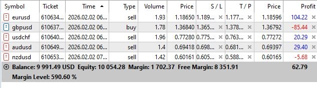
Overall, this system has yet to be tested. The first trades look like this:

Analysis of Results and Adaptation Patterns

The future of algorithmic trading lies not in finding the perfect algorithm, but in building adaptive systems capable of learning from their own experience and evolving alongside the market. The proposed architecture represents a step in this direction, but there is still ample room for further research and improvement.

# Adaptation results (April 2024)
initial_period = {
    'win_rate': 0.42,
    'sharpe': 0.65,
    'max_drawdown': 0.18,
    'rl_skip_ratio': 0.08,
    'seal_retrains': 0
}

after_adaptation = {
    'win_rate': 0.58,
    'sharpe': 1.35,
    'max_drawdown': 0.09,
    'rl_skip_ratio': 0.35,
    'seal_retrains': 2
}

An interesting pattern was observed around macroeconomic data releases. An hour before the release of the U.S. employment report, quantum entropy showed abnormally high values (over 4.5) even though the market appeared calm. The RL agent automatically learned to interpret this as a signal to exercise greater caution, increasing the frequency of REDUCE and SKIP actions. This behavior was not explicitly programmed — it emerged organically from adverse trading experience under highly volatile conditions.

By the end of the one-year testing period, the system had achieved stable metrics: win rate — 61%, Sharpe ratio — 1.67, and maximum drawdown — 12%. Critically, these results were obtained using data that had never been used in the initial training of the components. The system demonstrated an ability to learn online without interrupting trading and without catastrophic failures during periods of market regime shifts.

Limitations of the Approach and Directions for Development

Despite the encouraging results, the proposed system has a number of fundamental limitations that must be frankly acknowledged. First and foremost: in its current implementation, quantum encoding is performed on the classical Qiskit Aer simulator, which eliminates the potential quantum advantages of a real quantum processor. The question of whether a simulated quantum circuit offers a real advantage over an equivalent classical neural network with the same architecture remains open and requires further theoretical analysis.

The second limitation concerns the interpretability of the system. While a Q-learning agent with a tabular representation is completely transparent (you can directly inspect the Q-values and understand the logic behind its decisions), the DQN deep neural network remains a black box. Attempts to apply interpretation methods such as SHAP to financial data often yield conflicting results. For institutional traders who are required to explain every decision to regulators, this can be a critical obstacle.

The third limitation relates to computational requirements. Executing a parameterized quantum circuit with 2,048 measurements per trading cycle takes about 200 milliseconds on a modern processor. When trading dozens of instruments, this can introduce latency that is critical for high-frequency strategies. A move to real quantum hardware is not yet possible due to the high cost of and limited access to commercial quantum processors.

The fourth challenge is the amount of training data required to achieve stable SEAL operation. It may take several months of live trading to accumulate a statistically significant number of trading results, during which time the system will be suboptimal. Although historical data can be used for pretraining, this does not guarantee correct performance on future data due to non-stationarity.

Promising directions for development include integration with variational quantum algorithms to automatically optimize the quantum circuit architecture for the specifics of a particular market. Instead of a fixed sequence of gates, a variational quantum solver can be used to find the optimal parameterization that minimizes the entropy of the Q-function.

Another direction is hierarchical reinforcement learning with multiple levels of abstraction. The top level makes strategic decisions about the trading mode (trend following, mean reversion, or no trading); the middle level selects specific entry patterns; and the bottom level manages position sizing and stop-loss orders. Each level is trained separately but is coordinated through a common reward function.

Finally, integration with graph neural networks to model the interrelationships between various financial instruments can significantly enhance the market-state representation. The correlation structure of currency pairs, stocks, and commodities forms a dynamic graph whose topology changes depending on the macroeconomic regime. GNNs are capable of capturing these patterns and using them to improve predictions.

Conclusion and Practical Recommendations

This paper demonstrates the practical feasibility of building a self-adaptive trading system that combines the strengths of various machine learning approaches. Quantum encoding provides a compact, nonlinear market-state representation. Deep Q-learning makes it possible to optimize the sequence of trading decisions while taking long-term consequences into account. Large language models bring the ability to perform contextual analysis and generalize to new market regimes. The SEAL methodology ensures continuous self-learning without interrupting trading. A lightweight Q-learning filter acts as a metamodel that coordinates all the components.

It is critically important to understand that the system is not the “Holy Grail” of algorithmic trading. It cannot predict the future and does not guarantee a profit under all conditions. Its main advantage is the ability to adapt quickly when new market regimes emerge, minimizing the period of suboptimal performance.

For practical application, there are several recommendations to keep in mind. First, be sure to use a circuit breaker to stop trading in the event of consecutive losses. Second, start with minimal position sizes and gradually increase leverage only after sufficient statistics on successful operation have been accumulated. Third, regularly monitor not only financial metrics but also the system's internal parameters: the distribution of Q-values, the frequency of SEAL adaptations, and the dynamics of quantum entropy.

The system code is openly available for research purposes, but requires significant adaptation for commercial use. Specifically, integration with professional risk management systems is required, along with the addition of logic to support multiple accounts and the implementation of failover mechanisms in the event of infrastructure failures.