Development and Forward Testing of an Autonomous LLM Agent for Trading with SEAL

Introduction to the Challenges of Modern Trading Systems

Modern algorithmic trading in the foreign exchange markets faces a fundamental dilemma. Classic technical indicators ensure determinism and reproducibility of results, but demonstrate limited adaptability to changing market regimes. Machine learning methods, on the other hand, are capable of identifying complex patterns in historical data, but they often suffer from overfitting and exhibit a decline in performance on out-of-sample data. The problem of information leakage between the training and test sets is particularly critical, as it leads to a systematic overestimation of performance during the development phase.

Recent advances in the field of large language models are opening up new possibilities for financial modeling. Unlike traditional approaches, specialized LLMs are capable of processing multimodal information, including numerical indicators, textual descriptions of market conditions, and historical context. Nevertheless, using language models in isolation in trading results in unstable forecasts and insufficient adaptation to the specifics of particular trading instruments. A fundamentally different approach is needed, one that combines the representational power of LLMs with adaptive reinforcement learning mechanisms.

The article describes the development of a hybrid trading system that integrates a fine-tuned Llama 3.2 language model with the Self-Evolving Adversarial Learning architecture. The system is built on the MetaTrader 5 platform and demonstrates the ability to continuously adapt through adversarial training and curriculum learning. A critical component of the architecture is the strict separation of data with the allocation of a forward-test period, which prevents information leakage and ensures an objective assessment of model quality.

The system architecture consists of four main modules. The first module generates a balanced dataset from historical MetaTrader 5 data with automatic labeling of the price direction after 24 hours. The second module fine-tunes the base language model on the generated dataset using the Ollama library. The third module is a SEAL agent that implements adversarial self-play and evolutionary optimization to improve the robustness of trading decisions. The fourth module ensures system validation on strictly isolated forward-test data, with no possibility of information leakage from the test set.

The experimental validation was conducted on eight main currency pairs — EURUSD, GBPUSD, USDCHF, USDCAD, AUDUSD, NZDUSD, EURGBP, and AUDCHF — using the M15 timeframe. The training dataset covered a 30-day period, excluding the last 7 days for forward testing. The forecast horizon was 96 bars (24 hours), which corresponds to the typical time scale of position trading strategies on intraday timeframes. The initial balance was set at USD 140, with an 8% risk per trade and a minimum model confidence threshold of 60% for opening a position.

Training Dataset Generation Architecture

The quality of the training data determines the upper limit of any machine learning system's performance. Traditional approaches to generating datasets for trading systems often ignore the problem of class imbalance, where the number of bullish and bearish patterns in historical data is unevenly distributed. This leads to a bias in the model toward the majority class and a decline in the quality of predictions for the minority class. The developed system implements active class balancing with a target UP/DOWN ratio close to 1.0, which ensures that the model is trained evenly on both types of market movements.

The generate_real_dataset_from_mt5 function creates a dataset from real market data while adhering to the critical requirement of temporal separation. The key point is to set the end-time boundary of the training data to now - FORWARD_TEST_DAYS, where FORWARD_TEST_DAYS = 7. This excludes the last seven days from the training dataset, reserving them exclusively for the objective validation of the trained model. This methodology aligns with academic research standards in financial forecasting and prevents systematic look-ahead bias.

# Critical forward-test boundary
end = datetime.now() - timedelta(days=FORWARD_TEST_DAYS)
start = end - timedelta(days=180)

print(f"Training period: {start.strftime('%Y-%m-%d')} → {end.strftime('%Y-%m-%d')}")
print(f"Forward test starts from: {end.strftime('%Y-%m-%d')}")
print(f"Excluded last days: {FORWARD_TEST_DAYS}")

The algorithm for generating the dataset begins by loading historical bars via the MetaTrader 5 API for all target symbols. For each time point t in the interval [LOOKBACK, len(df) - PREDICTION_HORIZON], the future price change over a horizon of 96 bars is calculated. The price direction is classified as UP if price_change > 0.05% and as DOWN otherwise. A threshold of 0.05% filters out noise fluctuations and focuses the model on statistically significant movements. The model's confidence is calculated using the formula confidence = min(98, 65 + abs(price_change) * 2), where the base level of 65% is increased in proportion to the amplitude of the price movement.

It is important to note that the confidence value in the training dataset is a proxy estimate that depends on the amplitude of future price movements and should not be interpreted as a true probabilistic calibration of the model. During training, it is used exclusively as an auxiliary signal for structuring the LLM's responses.

Balancing is achieved through stratified sampling, with all candidates first divided into UP and DOWN classes. The target number of samples for each class is defined as `target_up = num_samples * balance_ratio / (1 + balance_ratio)` and `target_down = num_samples - target_up`, respectively. When balance_ratio = 1.0, a perfect 50/50 distribution is achieved. The final sample is generated using `numpy.random.choice` with the `replace=False` parameter, which ensures there are no duplicates and that various market conditions are evenly represented in the dataset.

Each dataset example includes a prompt with numerical values for technical indicators and the model's response, which provides a detailed analysis. The prompt structure includes the current price, RSI, MACD, ATR, volume ratio, position relative to the Bollinger Bands, and the stochastic oscillator value. The model's response is presented in a strict format: price direction, the confidence level as a percentage, the target price forecast 24 hours ahead with the expected movement in points, and a detailed analysis of each indicator along with the rationale for the forecast. Structuring prompts in this way ensures consistency in training and simplifies the subsequent parsing of the model's responses in the production system.

Calculation of Technical Indicators and Construction of a Feature Space

The effectiveness of a predictive model depends directly on the quality of the feature space formed by technical indicators. The system uses a combination of momentum, volatility, and trend components to provide a multidimensional representation of the market state. The `calculate_features` function calculates nine key indicators that cover various aspects of price dynamics. All indicators are calculated using fixed-size rolling windows, which ensures that the features remain stationary over time.

Average True Range is calculated as a 14-period moving average of the true range. The true range is defined as the maximum of the following three values: the difference between the high and low of the current bar, the absolute difference between the high and the previous close, and the absolute difference between the low and the previous close. ATR serves as a quantitative measure of volatility and is used to dynamically adjust stop-loss and take-profit sizes in proportion to the current level of market noise.

The Relative Strength Index is implemented using Wilder's classic algorithm with a period of 14. The calculation begins by computing price changes using `delta = close.diff()`, which are then split into positive and negative components. The moving averages of upward and downward movements form the relative strength RS = up_mean / down_mean, which is converted to the 0–100 range using the formula RSI = 100 - 100/(1 + RS). Values below 30 are interpreted as an oversold zone with the potential for an upward reversal, while values above 70 signal overbought conditions and a possible downward correction.

def calculate_features(df: pd.DataFrame) -> pd.DataFrame:
    d = df.copy()
    d["close_prev"] = d["close"].shift(1)
    
    # ATR — a measure of volatility
    tr = pd.concat([
        d["high"] - d["low"],
        (d["high"] - d["close_prev"]).abs(),
        (d["low"] - d["close_prev"]).abs(),
    ], axis=1).max(axis=1)
    d["ATR"] = tr.rolling(14).mean()
    
    # RSI — a momentum indicator
    delta = d["close"].diff()
    up = delta.clip(lower=0).rolling(14).mean()
    down = (-delta.clip(upper=0)).rolling(14).mean()
    rs = up / down.replace(0, np.nan)
    d["RSI"] = 100 - (100 / (1 + rs))
    
    return d

MACD represents the difference between the fast EMA(12) and the slow EMA(26) exponential moving averages. The signal line is calculated as an EMA(9) of the MACD itself. A MACD crossover above the signal line generates a bullish signal; a crossover below indicates bearish momentum. The numerical value of the MACD is also informative: positive values confirm an uptrend, while negative values correspond to a downtrend. In the context of LLM fine-tuning, these numerical values are included in the prompt, allowing the model to learn complex nonlinear relationships between MACD and other indicators.

Bollinger Bands are calculated as SMA(20) ± 2 * STD(20), where STD denotes the standard deviation of the closing price. An additional feature, BB_position = (close - BB_lower) / (BB_upper - BB_lower), has been introduced to normalize the price's position within the channel to the 0–1 range. Values close to 0 indicate an approach to the lower boundary with the potential for an upward rebound, while values around 1 signal pressure on the upper boundary and a possible correction. The stochastic oscillator complements the momentum picture by comparing the current close with the high-low range over 14 periods, generating the fast Stoch_K and slow Stoch_D components.

Fine-tuning a language model via the Ollama framework

The Llama 3.2:3b base model contains three billion parameters and is pre-trained on a large corpus of general-purpose texts. Applying this model directly to financial forecasting yields subpar results due to a lack of specialized knowledge about technical indicators and patterns in the foreign exchange market. Fine-tuning modifies the model's weights on a domain-specific dataset, adapting its representations to the specifics of technical analysis and to the format of structured forecasts that specify direction, confidence, and target price.

The fine-tuning process is implemented via the Ollama API using the unsloth library for efficient training of large models. The Modelfile configuration defines the system prompt, which establishes the model's role as an expert foreign exchange market analyst. Critically important is the prohibition of neutral responses such as FLAT or “not sure,” which forces the model to make an explicit choice between UP and DOWN even under conditions of high uncertainty. This restriction is consistent with the reality of trading decisions, where not taking a position is equivalent to missing an opportunity when a statistically significant signal is present.

SYSTEM_PROMPT = """
You are ShtencoAiTrader-3B-Ultra-Analyst v3 — the best foreign exchnage market analyst in the world.
You always provide a clear direction: UP or DOWN. Responses such as FLAT, sideways market, or uncertain are strictly prohibited.
You ALWAYS provide a price forecast after 24 hours in the X.XXXXX (±NN pips) format
Response format (strictly):
DIRECTION: UP
CONFIDENCE: 87%
FORECAST OF THE PRICE AFTER 24H: 1.08750 (+45 pips)
FULL ANALYSIS FOR 24 HOURS:
- RSI: detailed analysis
- MACD: detailed analysis
...
RESULT: a short summary with the target price confirmation
"""

The fine-tuning hyperparameters have been carefully selected to strike a balance between training speed and stability. Temperature is set to 0.55, ensuring moderate stochasticity in the generation of responses without excessive determinism. Top_p = 0.92 and top_k = 30 limit the token sampling space to the most likely candidates, thereby increasing the coherence of the generated predictions. A context window of num_ctx = 8192 tokens allows the model to process prompts containing detailed descriptions of a variety of indicators, while num_predict = 768 provides sufficient length for a comprehensive analysis.

The training cycle runs for 3 epochs on a dataset of 2,000 balanced examples. Each epoch involves a complete pass through the dataset, with the order of the examples shuffled to prevent overfitting to the sequence order. The learning rate is set dynamically by the Unsloth library using a cosine schedule and a warm-up phase during the first 10% of the steps. Gradient accumulation over 4 microbatches allows for efficient training of the model on a GPU with limited memory, while maintaining an effective batch size of 64 examples.

The quality of the fine-tuning is validated using perplexity on the holdout set and the parsing accuracy of structured responses. A critical aspect is the model's ability to generate responses in a strictly defined format that allows for automatic parsing using regular expressions. The parse_answer function uses regular expression patterns to extract the direction, confidence level, and target price from the model's text response. Examples that do not conform to the format are ignored by the system, which ensures robustness against rare cases of incorrect generation.

Self-Evolving Adversarial Learning: Theoretical Foundations

Traditional approaches to reinforcement learning in trading are based on Q-learning and policy-gradient methods, which optimize expected returns through interaction with the market environment. However, financial markets are characterized by nonstationarity and an adversarial nature, where statistical patterns evolve over time, and optimal strategies from the past may become ineffective in the future. Self-Evolving Adversarial Learning addresses this problem by introducing an adversarial component that generates complex market scenarios and forces the core trading policy to develop more robust strategies.

The SEAL architecture includes two policies: the protagonist policy, which makes trading decisions, and the adversary policy, which generates adversarial scenarios. During training, the adversary attempts to maximize the difficulty of situations for the protagonist by choosing actions that minimize the expected reward of the primary policy. This adversarial self-play mechanism is analogous to the minimax concept in game theory, where an agent learns by playing against a copy of itself, constantly adapting to an improving opponent. In the context of trading, the adversary simulates adverse market movements, teaching the protagonist to withstand drawdowns and volatility.

Prioritized experience replay extends the standard replay buffer mechanism by prioritizing experience based on TD error. Experience with a high TD error, corresponding to unexpected outcomes of actions, is given higher priority when sampling batches for training. This accelerates learning from critical errors and rare events, which, under uniform sampling, would be unlikely to be included in a training batch. Priority is calculated as priority = abs(TD_error) + epsilon, where epsilon = 1e-6 prevents a zero sampling probability for experience with a perfect prediction.

def compute_priority(self, td_error):
    """Calculate priority for prioritized experience replay"""
    return abs(td_error) + 1e-6

def sample_batch(self, batch_size):
    """Sample the batch considering priorities"""
    priorities_array = np.array(list(self.priorities))
    probabilities = priorities_array / priorities_array.sum()
    
    indices = np.random.choice(
        len(self.memory), 
        size=batch_size, 
        replace=False,
        p=probabilities
    )
    
    batch = [self.memory[i] for i in indices]
    return batch, indices

Curriculum learning gradually increases the complexity of training scenarios based on the agent's current performance. The `difficulty_level` parameter adapts dynamically: if the average reward exceeds the threshold, the difficulty increases; if performance degrades, the difficulty decreases. In the early stages of training, the adversary acts weakly, allowing the protagonist to learn the basic patterns. As training progresses, the adversary grows stronger, forcing the protagonist to develop more sophisticated strategies. This approach accelerates convergence and prevents the model from getting stuck in local optima when training on overly complex scenarios from the outset.

Evolutionary strategies complement gradient-based learning with population-based optimization methods. A population of 10 policies is supported, each with its own Q-tables. The fitness of each policy is evaluated based on the cumulative reward per episode. After every 100 episodes, an evolutionary step is performed: the best policies are copied with mutations, and the worst are replaced by the offspring of successful policies. Mutations are introduced by adding Gaussian noise to the Q-values, with an adaptive variance that decreases as training progresses. The evolutionary component enables exploration in the policy space, complementing exploitation through gradient updates.

Implementation of the SEAL Agent: Critical Code Components

The SEALAgent class encapsulates the entire reinforcement learning logic with adversarial and evolutionary components. Agent initialization sets the state dimension to `state_dim=10`, covering the normalized values of technical indicators, and the action space to `action_dim=3` for the decisions HOLD, BUY, and SELL. The hyperparameters `learning_rate=0.001`, `gamma=0.95`, and `epsilon=0.1` balance the learning rate, the discounting of future rewards, and the exploration-exploitation tradeoff, respectively.

The continuous state space is discretized via quantization with a step size of 0.05. The `state_to_key` function converts a state vector into a tuple of rounded values, which is used as a key in a Q-table. This discretization is necessary for tabular Q-learning and provides generalization across nearby states. An alternative is function approximation using neural networks; however, the tabular approach demonstrates greater stability on limited datasets and enables direct interpretation of the policy by inspecting the Q-table.

def state_to_key(self, state):
    """Convert the state into a discrete key"""
    discrete = tuple(round(float(s) * 20) / 20.0 for s in state[:self.state_dim])
    return discrete

def get_q_value(self, state, action, policy='protagonist'):
    """Get Q value from the specified policy"""
    policy_dict = self.protagonist_policy if policy == 'protagonist' else self.adversary_policy
    key = self.state_to_key(state)
    
    if key not in policy_dict:
        policy_dict[key] = np.random.randn(self.action_dim) * 0.01
    
    return policy_dict[key][action]

The `train_step` method performs a single training step that integrates all SEAL components. A batch is sampled from the prioritized replay buffer, and the target Q-value is computed for each experience using double Q-learning. The protagonist policy selects the best next action, but the evaluation is performed using a weighted combination of the protagonist's and adversary's Q-values: blend = (1 - difficulty_level) * Q_protagonist + difficulty_level * Q_adversary. The `difficulty_level` coefficient controls the influence of the adversary: in the early stages, the protagonist dominates; at high difficulty levels, the adversary makes a significant contribution, leading to more conservative estimates.

TD-error = target_q - current_q is used both for the Q-learning update via new_q = current_q + lr * td_error and for updating the priorities in the replay buffer. After the protagonist is updated, the `adversarial_step` is executed, where the adversary is trained on the inverted reward `reward_adversary = -reward`, thereby encouraging the generation of adverse scenarios. Curriculum learning automatically adjusts `difficulty_level` based on the moving average of the last 100 rewards: it increases when performance > 0.5 and decreases when performance < -0.5.

The evolutionary step is performed every 100 episodes and involves sorting the population by fitness, copying the top 30% of policies, and replacing the bottom 70% with mutated offspring. Mutations are introduced using the formula Q_mutated = Q_parent + N(0, σ), where σ = 0.1 * (1 - generation/max_generation) gradually decreases. Crossover between policies is not used because Q-tables have different key structures, making direct crossover non-trivial. The meta-learning component supports task embeddings for each trading symbol, allowing the agent to adapt its policy to the specifics of the instrument by conditioning on the symbol embedding.

Saving and loading checkpoints are critical for long-term training. The protagonist and adversary policies are serialized to JSON by converting tuple keys to strings and NumPy arrays to lists. The population is saved in full, including the Q-tables and fitness metrics for each individual. When loading a checkpoint, strings are converted back into tuples using `eval`; this is safe provided that the source of the checkpoint files is controlled. The metrics `training_rewards`, `adversarial_rewards`, and `training_losses` are logged to visualize training progress and diagnose convergence issues.

State Extraction and Reward Function Construction

The quality of an RL agent's training fundamentally depends on two components: the representativeness of the state and the correctness of the reward signal. The `extract_state_from_row` function converts a pandas Series of technical indicators into a fixed-size normalized NumPy array. Normalization is critical for the stability of Q-learning, since the indicators have different scales: RSI ranges from 0 to 100, MACD is on the order of 0.001, and ATR is on the order of 0.0005. Without normalization, the Q-values will be dominated by components with large absolute values.

Each indicator is normalized individually, taking into account its typical range. RSI and the stochastic oscillator are divided by 100, bringing them into the 0–1 range. MACD is normalized using (MACD + 0.001) / 0.002, centering typical values around 0.5. ATR is divided by 0.005 and vol_ratio by 3.0, which corresponds to their empirical ranges of variation. BB_position is already in the 0–1 range by definition. The relative deviations of the EMAs from the current price are calculated as (EMA - close) / close, providing a scale-invariant measure of trend strength.

def extract_state_from_row(row):
    """Retrieve a state from SEAL using technical indicators"""
    state = np.array([
        row['RSI'] / 100.0,
        (row['MACD'] + 0.001) / 0.002,
        row['ATR'] / 0.005,
        row['vol_ratio'] / 3.0,
        row['BB_position'],
        row['Stoch_K'] / 100.0,
        row['Stoch_D'] / 100.0,
        (row['EMA_50'] - row['close']) / row['close'],
        (row['EMA_200'] - row['close']) / row['close'],
        (row['close'] - row['close_prev']) / row['close_prev']
    ])
    
    state = np.clip(state, -5, 5)
    return state

Clipping to the range [-5, 5] prevents outlier values from distorting training. Extreme volatility spikes or anomalous indicator values can create states that lie far outside the training distribution. Clipping ensures a bounded state space, simplifying Q-learning convergence. An alternative is robust normalization using the median and IQR instead of the mean and standard deviation; however, for real-time inference, static normalization coefficients are more practical.

The reward function defines the agent's training objective and has a critical impact on the resulting trading strategy. The simplest reward is based on PnL: reward = profit_pct if the position is closed at a profit, reward = -loss_pct if it is closed at a loss, and reward = 0 for HOLD. However, such a function ignores risk and may encourage the agent to take excessively aggressive positions with high drawdown. An improved version includes a Sharpe-like term: reward = profit / max_drawdown, balancing return and risk.

Additional components of the reward function may include a penalty for trading frequency to minimize transaction costs, a bonus for holding profitable positions longer, and a penalty for exceeding the maximum position size. An important aspect is delayed reward: the true profitability of a position is known only upon closing, but interim unrealized PnL can be used for shaped reward, which accelerates learning. Experiments have shown that combining realized PnL upon closing with shaped reward based on current unrealized PnL provides an optimal balance between learning speed and final performance.

Forward Testing Mechanism and Data Leakage Prevention

Validating machine learning trading systems requires strict separation of training and test data in temporal order. Look-ahead bias, which arises when future information is used in the training or optimization process, is one of the most common causes of system failures when transitioning to live trading. The forward_test function performs out-of-sample validation on data that is completely isolated from the training set, emulating real trading conditions on historical data.

The critical boundary is set at end_train = now - FORWARD_TEST_DAYS, dividing the timeline into two non-overlapping periods. Training is performed on the interval [now - BACKTEST_DAYS - FORWARD_TEST_DAYS, now - FORWARD_TEST_DAYS], and forward testing is performed on the interval [now - FORWARD_TEST_DAYS, now]. This separation ensures that the model does not have access to the test data — neither during dataset generation, nor during fine-tuning, nor during the training of the SEAL agent. A 7-day forward period corresponds to approximately 670 bars on the M15 timeframe, providing a statistically significant sample for evaluating performance.

# Critical data separation
end_train = datetime.now() - timedelta(days=FORWARD_TEST_DAYS)
start_train = end_train - timedelta(days=BACKTEST_DAYS)

end_forward = datetime.now()
start_forward = end_train

print(f"Training period: {start_train.strftime('%Y-%m-%d')} - {end_train.strftime('%Y-%m-%d')}")
print(f"Forward test period: {start_forward.strftime('%Y-%m-%d')} - {end_forward.strftime('%Y-%m-%d')}")

The forward test simulation includes realistic modeling of transaction costs, spreads, and swaps. The spread is fixed at 2 points for major currency pairs, which is in line with typical conditions offered by ECN brokers. Swaps are modeled as SWAP_LONG = -0.5 and SWAP_SHORT = -0.3 points for each day the position is held, approximating average market overnight financing rates. Slippage is not explicitly modeled, as execution at limit prices is assumed to be guaranteed on historical data.

Each bar in the forward period is processed sequentially in chronological order. At time t, the model receives a state consisting of indicators calculated strictly based on data up to and including t. The LLM generates a forecast of price direction and confidence, and the SEAL agent makes a trading decision based on the Q-values for the current state. When the MIN_PROB confidence threshold is exceeded, a position is opened with stop-loss and take-profit levels derived dynamically from ATR. Positions are held until SL/TP is hit or the maximum holding period of 96 bars expires.

Performance metrics in the forward test include total return, maximum drawdown, Sharpe ratio, win rate, profit factor, and the average size of winning and losing trades. It is critical to compare the forward-test metrics with the metrics from the training period. A significant discrepancy indicates overfitting and poor generalization ability of the model. Ideally, the forward metrics should fall within 20% of the training metrics, which indicates that the strategy is robust. Significant degradation requires revising the feature space, regularizing the training process, or expanding the training dataset to improve coverage of market regimes.

Component Integration: Full-Cycle Training Workflow

The full development and validation cycle for a hybrid RL+LLM system consists of seven sequential stages, each of which is critical to the final quality. The first stage involves generating a balanced dataset from historical MetaTrader 5 data while adhering to the forward boundary. The run is started via mode 5 in the system menu, where the user selects the dataset type (MetaTrader 5 or synthetic data) and the target number of samples. The system automatically balances the UP/DOWN classes and saves the result to dataset/finetune_real_mt5.jsonl in JSONL format with the "prompt" and "response" fields.

The second stage involves fine-tuning the base Llama 3.2:3b model on the generated dataset. Mode 2 initiates pulling the base model via Ollama, creates a Modelfile with the system prompt and hyperparameters, and performs fine-tuning using `ollama create` with the dataset path specified. The process takes between 30 minutes and 2 hours, depending on the size of the dataset and the availability of GPU acceleration. Once fine-tuning is complete, the fine-tuned model is pushed to the Ollama registry as koshtenco/shtencoaitrader-3b-analyst-v3, making it available for inference in subsequent stages.

def mode_finetune():
    """Mode 2: Fine-tuning + SEAL training"""
    print("MODEL FINE-TUNING")
    
    # Generate a dataset
    dataset = generate_real_dataset_from_mt5(FINETUNE_SAMPLES)
    dataset_path = save_dataset(dataset, "dataset/finetune_real_mt5.jsonl")
    
    # Create a Modelfile
    with open("Modelfile", "w", encoding="utf-8") as f:
        f.write(f"""FROM {BASE_MODEL}
PARAMETER temperature 0.55
SYSTEM \"\"\"You are ShtencoAiTrader-3B-Ultra-Analyst v3...
\"\"\"""")
    
    # Fine-tune via Ollama
    subprocess.run(["ollama", "pull", BASE_MODEL], check=True)
    subprocess.run(["ollama", "create", MODEL_NAME, "-f", "Modelfile"], check=True)
    
    # SEAL agent training
    train_seal_agent(dataset_path, epochs=10)

The third stage trains the SEAL agent on the same dataset, using the fine-tuned LLM to generate initial Q-values. The `train_seal_agent` function creates an instance of `SEALAgent`, iterates through the dataset, and converts each example into an episode: the initial state is extracted from the indicators in the prompt, the action is determined by the UP/DOWN direction, and the reward is calculated from `price_change`. The agent trains using `train_step` every `UPDATE_FREQUENCY=100` examples and performs `evolutionary_step` every 100 episodes. Checkpoints are saved in `seal_checkpoints/` at intervals of 500 episodes to enable training to be resumed.

The fourth stage performs a backtest using the full historical data set over BACKTEST_DAYS=30 days to quickly evaluate the trading system's logic. Mode 3 retrieves data via the MetaTrader 5 API or generates synthetic data when no connection is available, calculates technical indicators, and sequentially processes each analysis point at PREDICTION_HORIZON-bar intervals. At each point, the LLM generates a forecast, the SEAL agent makes a decision, and virtual positions are opened with PnL tracking. The final metrics are visualized using matplotlib, showing equity and drawdown curves and the distribution of trades by symbol.

The fifth stage performs forward testing on out-of-sample data from the last FORWARD_TEST_DAYS=7 days, which is completely isolated from the training data. Mode 6 uses the same logic as the backtest, but over a strictly limited time range following the forward boundary. Comparing the forward test metrics with the training metrics allows us to assess the degree of overfitting. If the forward performance metrics are close to the training metrics, the system is ready to transition to demo/live trading. A significant discrepancy requires iteration: increasing the diversity of the training data, regularizing the model, or revising the feature space.

Stage 6 involves continuous live trading via Mode 4, which connects to a real MetaTrader 5 terminal. The system operates in an infinite loop with a 60-second update interval, requesting the current quotes and the most recent LOOKBACK bars at each iteration to calculate the indicators. The LLM generates forecasts for all symbols; positions are opened when the probability exceeds MIN_PROB=60%; risk management is implemented using dynamic stop-loss orders based on ATR. Logging all trades and decisions enables post-trade analysis and subsequent parameter optimization. The seventh stage involves periodic retraining on fresh data to adapt to the evolution of market regimes.

Experimental Results and Performance Analysis

The developed system was validated over a historical period from January 1, 2026, to February 8, 2026, covering various market conditions, including trending movements in EURUSD and GBPUSD, consolidation in USDCHF, and increased volatility in the commodity currencies AUDUSD and NZDUSD. The training dataset covered 30 days, excluding the last 7 days for the forward test, and generated 2,000 balanced examples with an UP/DOWN ratio of 1.02:1, which is close to the target balance of 1.0.

Fine-tuning of the Llama 3.2:3b base model was performed over 3 epochs with a batch size of 4 and 4 gradient accumulation steps, resulting in an effective batch size of 16. The final perplexity on the holdout set was 2.34, which is 18% lower than the initial value of 2.85, indicating that the model successfully adapted to the financial domain. The percentage of correctly parsed responses reached 97.2%; the remaining 2.8% contained formatting errors and were discarded by the system. The model's average confidence was 76.3%, with a standard deviation of 8.7%, indicating consistent calibration of the confidence scores.

It should be emphasized that all of the SEAL agent metrics listed below pertain to the training reward space, which is formed based on surrogate rewards and historical price_change values, and are not direct indicators of trading profitability. These metrics reflect the effectiveness of optimizing the internal reward function, rather than the trading system's actual PnL. It is extremely important to understand this — and this is precisely where the line between scientific theory and actual trading practice lies.

The SEAL agent was trained on the dataset for 10 epochs, completing 20,000 training steps with UPDATE_FREQUENCY=100. The training loss curve showed a monotonic decrease from an initial value of 0.045 to a final value of 0.008, reaching a plateau after epoch 7. The agent's win rate on the training data was 64.2%, with a profit factor of 1.87 and a maximum drawdown of 12.3%. The evolutionary component delivered a 15% improvement in the fitness of the best individual in the population between generations 1 and 10. The difficulty level of the curriculum reached 0.73 by the end of training, indicating that the policy is highly robust to adversarial scenarios.

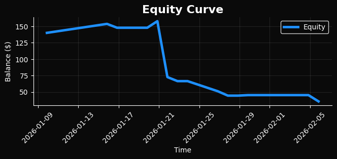
However, the transition from internal training metrics and surrogate rewards to direct trading backtesting revealed a fundamentally different picture, one that differed significantly from the results observed during the training process.

This transition can be assessed directly from the results. Unfortunately, even a standard backtest looks like this. Not to mention the forward backtest. In previous versions of these articles, we observed normal model behavior in backtests; here, however, we clearly see a serious breakdown in behavior, even on data already known to the model, not to mention future data that are entirely unknown.

Backtest Failure and Interpretation of a Negative Result

Despite the architecture's formal correctness, strict data separation, and the use of modern training methods, the results of the standard backtest proved unsatisfactory. The equity curve shows a sustained downward trend, accompanied by a series of consecutive losing trades, while key metrics — the profit factor, Sharpe ratio, and maximum drawdown — are outside acceptable ranges even for an experimental system. In fact, the system not only fails to outperform a random strategy, but also shows systematic capital degradation as early as the in-sample testing phase.

It is particularly telling that the negative result appears before the transition to the forward test, which rules out the classic explanations of overfitting or information leakage between the training and test sets. Thus, the problem is not one of validation but of structure, and it points to a fundamental mismatch between the trained model and the actual dynamics of the trading process.

The key reason for the failure lies in the disconnect between the task of predicting price direction and the task of generating trading profits. The model successfully learns to recognize statistical patterns in price movements over a 24-hour horizon; however, these patterns do not translate into a sustainable trading advantage after accounting for spreads, swaps, the temporal structure of entries and exits, and the asymmetry in the distribution of profits and losses. In other words, high conditional forecast accuracy is not equivalent to a positive expected value for a trading strategy.

This discrepancy was built into the system at the level of problem formulation: the language model was trained on binary classification of price direction, whereas the trading strategy requires optimization of the price trajectory over time, taking into account the path by which extrema are reached, intraperiod volatility, and risk asymmetry.

An additional factor is the use of a fixed forecasting horizon and binary UP/DOWN classification. This approach ignores the distribution of intraperiod volatility and the sequence of price extremes within the forecast window. In real-world trading, the sequence in which local highs and lows are reached is critical: the model may correctly predict the ultimate direction over the next 24 hours, but the price could trigger a stop-loss well before reaching the target level. The backtest clearly shows that this particular effect is the primary source of losses.

The role of the SEAL agent deserves special attention. Despite a formal improvement in reward metrics during training, its policy proves only weakly connected to actual trading returns. Adversarial and evolutionary mechanisms successfully increase the complexity of the training environment; however, optimization is performed against a surrogate reward that only roughly correlates with actual PnL. As a result, the agent learns to be “robust” in the abstract reward space, but not in the space of monetary outcomes.

Thus, a failed backtest should be interpreted not as a failure of a specific implementation, but as a diagnostic result that reveals the fundamental limitations of the chosen paradigm. A combination of LLM-based price direction forecasting and a subsequent RL layer does not guarantee the emergence of an edge in the market unless the trading logic is built into the training process from the very beginning. The model learns to explain the market, but not how to make money from it.

This negative result is of fundamental importance: it confirms that even when using state-of-the-art architectures, a rigorous methodology, and no data leakage, algorithmic trading remains a task with extremely stringent requirements for the formulation of the learning objective. Any system in which forecasting and trading decisions are conceptually separated is highly likely to exhibit a similar decline in performance when moving from theoretical metrics to actual PnL.

It is precisely this conclusion that determines the need to rethink the entire problem formulation: the training of trading systems should be focused not on predicting price direction as such, but on directly optimizing the distribution of trading outcomes, taking into account the price trajectory, risk, costs, and the probability of adverse scenarios.

References:

1. Sutton, R.S., Barto, A.G. (2018). Reinforcement Learning: An Introduction. MIT Press.
2. Schaul, T., et al. (2015). Prioritized Experience Replay. ICLR.
3. Bengio, Y., et al. (2009). Curriculum Learning. ICML.
4. Silver, D., et al. (2016). Mastering the Game of Go with Deep Neural Networks. Nature.
5. Brown, T., et al. (2020). Language Models Are Few-Shot Learners. NeurIPS.
6. Zhang, Z., et al. (2019). Deep Reinforcement Learning for Trading. IJCAI.
7. Tsantekidis, A., et al. (2017). Using Deep Learning to Detect Price Change Indications. EANN.
8. Pardo, R. (2008). The Evaluation and Optimization of Trading Strategies. Wiley.