Trading Options Without Options (Part 3): Complex Option Strategies

Introduction

In the previous article in this series, we examined basic options strategies and tested how they performed in the real market. We created an EA that implements an options strategy. Now it is time to examine the strategies used by options traders in practice and put them into action. This will let us explore the new opportunities offered by options trading.

Visualization of option levels

Before moving on, let's add the ability to display current option levels to the EA. To facilitate visual monitoring of the trading process, it would be helpful to see, in the terminal, the position of the underlying asset’s current price relative to the option levels used in the simulation. In addition, we will test the option strategies discussed in Part 2.

We will display option levels as lines extending from the start of the day to the current time. It would also be helpful to see the strike prices displayed on the terminal screen. First, let's define the CalculateLevelPrice method. In fact, this method performs the inverse operation — it calculates the relative price based on a given option delta value. From the relative price, we will obtain a specific absolute price value for each option level.

Let's add the TOptionConstructionBase::CalculateUpLevelPrice and TOptionConstructionBase::CalculateDnLevelPrice abstract methods and define them in the derived classes. Have a closer look at these calculation methods.

Why are there two methods? This is done because the delta will differ depending on whether the price of the underlying asset is above or below the strike price. That is why we we account for all possible cases. The arguments for the TOptionConstructionBase::CalculateUpLevelPrice and TOptionConstructionBase::CalculateDnLevelPrice methods are as follows:

• _strike_price — strike price;
• _norm_price — the price normalized to a volatility range;
• _limit_price — the maximum/minimum price for an interval when searching using the bisection method (generally equal to the normalization price) — above/below the strike price, respectively;
• _target_delta — the target delta value of the option structure the price level is being searched for.

NOTE:

Since the sigmoid function approaches zero and one (or negative one) exponentially but never actually reaches them, we use values close to zero and one to explicitly define the option levels corresponding to the zero level and the maximum (for example, the tenth).

For the zero level, we take a delta equal to _norm_zero_level with the appropriate sign. For the maximum level, we use a delta value of ±0.96 (determined empirically) with the appropriate sign. In this case, we will limit the range of the _norm_zero_level value to between 0.01 and 0.05 (note that the first level of option emulation corresponds to a delta of ±0.1).

The code for these methods is as follows:

// ---------------------------------------------------------------------
//  Calculate price levels corresponding to the upper option levels:
// ---------------------------------------------------------------------
void CalculateUpPriceLevels(const double _norm_zero_level, double& _strike_price[], double& _norm_price[], double& _limit_price[]) override
{
  //  If the array has zero size, there are no levels:
  if(ArraySize(this.up_level_values_Array) == 0)
  {
    ArrayResize(this.up_price_level_Array, 0);
      
    return;
  }

  //  Zero and last levels are set separately:
  this.up_level_values_Array[0] = _norm_zero_level;
  this.up_level_values_Array[10] = 0.96;

  ArrayResize(this.up_price_level_Array, this.emulation_levels_number + 1);
  
  //  Main levels:
  for (int i = 0; i <= this.emulation_levels_number; i++)
  {
    this.up_price_level_Array[i] = this.CalculateUpLevelPrice(_strike_price[1], _norm_price[1], _limit_price[1], this.up_level_values_Array[i]);
  }
}
// ---------------------------------------------------------------------
//  Calculate price level for the specified normalized delta:
// ---------------------------------------------------------------------
double CalculateUpLevelPrice(const double _strike_price, const double _norm_price, const double _limit_price, const double _target_delta) override
{
  double low_limit = _strike_price;
  double up_limit = _limit_price;
  double half_point = (low_limit + up_limit) / 2.0;

  double curr_point = this.UpdateOptionConstructionDelta(half_point);

  //  Till the error (segment length) exceeds the specified one, continue dividing the segment:
  while (MathAbs(search_point - _target_delta) > this.tolerance)
  {
    //  Evaluate the position of the current (average) point relative to the target one:
    if(curr_point > _target_delta)
    {
      up_limit = half_point;
    }
    else if(fc < _target_delta)
    {
      low_limit = half_point;
    }
    else
    {
      return (half_point);
    }

    //  Next middle point on the segment:
    half_point = (low_limit + up_limit) / 2.0;
    curr_point = this.UpdateOptionConstructionDelta(half_point);
  }

  return (low_limit + up_limit) / 2.0;
}

The TOptionConstructionBase::CalculateUpPriceLevels method iterates through all option emulation level values and calls the TOptionConstructionBase::CalculateUpLevelPrice method, which calculates the price corresponding to the specified delta.

For this calculation, we will use the bisection method (dichotomy method) to avoid solving the sigmoid equation analytically. This is possible because the sigmoid is a continuous, monotonic function of price, and within the working range of the option structure (where the main rebalancing occurs), the sum of the sigmoids is also monotonic.

Figure 1 schematically illustrates the iterative process (the first three steps — Step 1, ..., Step 3) for finding a point within a segment (the value target in Fig. 1). The method involves sequentially determining in which half of the interval [up_limit; low_limit] the target point of interest is located. Once we have determined this, we change the segment's boundary (in this case, the up_limit upper boundary in the first three steps) to the midpoint of the interval:

half_point = (up_limit + low_limit) / 2 ---> up_limit = half_point

Repeat this procedure until the length of the segment equal to (up_limit - low_limit) becomes less than or equal to the specified _tolerance.

In this case, the value we are looking for will be equal to the last half_point value. The value we are looking for will be no farther from target than the specified precision. This procedure for calculating option levels will be called once a day at the start of a new day or when the EA starts.

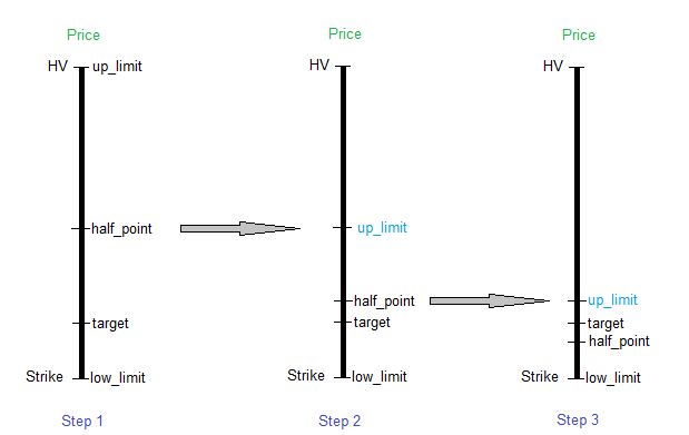
Fig. 1: Algorithm for finding a point within a line segment

After applying the CalculateUpLevelPrice method to all option level values (0, 1, ..., 10), we obtain an array of price values corresponding to these levels — option levels above the strike price. To calculate option levels below the strike price, the CalculateDnLevelPrice method is used (see the OptionEmulatorA3.mqh file). The search is performed in the same way — the difference is that the option levels are plotted downward along the price scale from the strike price. In general, the lower and upper levels are not necessarily symmetrical.

Now let's visualize the option levels on the MetaTrader 5 terminal chart. To do this, we will create two classes: the one that encapsulates the level itself, and the one for manipulating the list of levels. The level visualization class is shown below:

// =====================================================================
//  Base class of the option level - derived from CObject:
// =====================================================================
#define DESTROY_OBJECT(object)  { if(CheckPointer(object) == POINTER_DYNAMIC) delete(object); }
// ---------------------------------------------------------------------
class TPriceLevelBase : public CObject
{
private:
  long    chart_id;
  int     window;
  string  trend_name;
  string  text_name;
  double  price;

protected:
  CChartObjectTrend*  trend;
  CChartObjectText*   text;

public:
  // ---------------------------------------------------------------------
  //  Constructor:
  // ---------------------------------------------------------------------
  TPriceLevelBase(long _chart_id, const int _window)
  :
  chart_id(_chart_id),
  window(_window),
  trend_name(GetUniqIdentString()),
  text_name(GetUniqIdentString()),
  CObject()
  {
    this.trend = new CChartObjectTrend();
    this.text = new CChartObjectText();
  }
  // ---------------------------------------------------------------------
  //  Destructor:
  // ---------------------------------------------------------------------
  ~TPriceLevelBase()
  {
    DESTROY_OBJECT(this.trend);
    DESTROY_OBJECT(this.text);
  }
  // ---------------------------------------------------------------------
  //  Create object:
  // ---------------------------------------------------------------------
  void  Create(const datetime _time1, const datetime _time2, const double _price, const string _text, const int _font_size, const color _color1, const color _color2, const int _width, const ENUM_LINE_STYLE _style)
  {
    this.price = _price;
    this.trend.Background(false);
    this.trend.Create(this.chart_id, this.trend_name, this.window, _time1, _price, _time2, _price);
    this.trend.Width(_width);
    this.trend.Style(_style);
    this.trend.RayRight(false);
    this.trend.Color(_color1);

    this.text.Create(this.chart_id, this.text_name, this.window, _time2 + 15 * 60, _price);
    this.text.Description(_text);
    this.text.FontSize(_font_size);
    this.text.Anchor(ANCHOR_LEFT);
    this.text.Background(false);
    this.text.Color(_color2);
  }
  // ---------------------------------------------------------------------
  //  Update the object:
  // ---------------------------------------------------------------------
  void  Update(const datetime _time)
  {
    this.text.SetPoint(0, _time + 15 * 60, this.price);
    this.trend.SetPoint(1, _time, this.price);
  }
};
// ---------------------------------------------------------------------

As we can see, the TPriceLevelBase class is derived from the standard CObject class. This is done so that a standard class can be used to manipulate the list. More on this below. A "level" object is a horizontal segment (line) extending from the current day's opening time to the current time within the day. To the right of the line, we will display a text label — the level number.

The data members that encapsulate the properties of the "level" object are the standard properties of the "line" and "text label" graphical objects on the MetaTrader 5 terminal chart. Their purpose is as follows:

• long chart_id — the ID of the chart the graphical object is located on;
• int window — the ID of the subwindow on the chart containing the graphical object; in this case, zero for the main chart window;
• string trend_name — the name of the "line" object to identify it among other similar objects on the chart;
• string text_name — the name of the "text" object to identify it among other similar objects on the chart;
• double price — the value of the price level the objects are located at — a horizontal segment and a text label;

• CChartObjectTrend* trend — the pointer to the "line" chart object from the MetaTrader 5 standard library;
• CChartObjectText* text — the pointer to the "text label" graphical object from the MetaTrader 5 standard library.

The levels are updated when a new bar appears on the MetaTrader 5 chart. At the start of a new day, the old levels are removed and new ones begin to be plotted for the current day. Before that, the historical volatility (HV) is recalculated for the new day.

Intraday levels are updated when the TPriceLevelBase::Update(const datetime _time) method is called; its argument is the open time of the current bar. The time coordinate of the text label is shifted further to the right so that it does not overlap with the level line.

The class for manipulating the TVisualPriceLevels list is shown below:

// =====================================================================
//  Visualize rebalancing levels for an option structure:
// =====================================================================
class TVisualPriceLevels : public CList
{
private:
  long  chart_id;
  int   window;

public:
  // ---------------------------------------------------------------------
  //  Destructor:
  // ---------------------------------------------------------------------
  ~TVisualPriceLevels()
  {
    this.Clear();
  }
  // ---------------------------------------------------------------------
  //  Constructor:
  // ---------------------------------------------------------------------
  TVisualPriceLevels(const long _chart_id, const int _window)
  :
  chart_id(_chart_id),
  window(_window),
  CList()
  {
    this.FreeMode(true);
  }
  // ---------------------------------------------------------------------
  //  Add a level:
  // ---------------------------------------------------------------------
  void  AddLevel(const datetime _time1, const datetime _time2, const double _price, const string _text, const int _font_size, const color _color1, const color _color2, const int _width, const ENUM_LINE_STYLE _style)
  {
    TPriceLevelBase* new_level = new TPriceLevelBase(this.chart_id, this.window);
    new_level.Create(_time1, _time2, _price, _text, _font_size, _color1, _color2, _width, _style);
    this.Add(new_level);
  }
  // ---------------------------------------------------------------------
  //  Update levels:
  // ---------------------------------------------------------------------
  void  Update(const datetime _time)
  {
    if(this.Total() > 0)
    {
      TPriceLevelBase* trend = this.GetFirstNode();
      while(trend != NULL)
      {
        trend.Update(_time);
        trend = this.GetNextNode();
      }
    }
  }
};
// ---------------------------------------------------------------------

As in the TPriceLevelBase class, there is also a method here called TVisualPriceLevels::Update(const datetime _time), which updates all levels added to the list by iterating through the objects and calling the TPriceLevelBase::Update(const datetime _time) method on each object.

The TVisualPriceLevels::AddLevel method has been added, with parameters that specify the position and style of the line (for an optional level) or text label. This method creates an object of TPriceLevelBase type and adds it to the list by calling the CList::Add method of the standard CList class.

In addition, we will add new inputs to the main EA file ("Article3-OptionTrader.mq5") to set the properties of the levels displayed on the screen — the text label color, line color, and line style. We can set the parameters for lines and text labels separately for the strike and the upward/downward rebalancing levels.

// ---------------------------------------------------------------------
input color     StrikeLevelTextColor = clrYellow;                     // Strike Level Text Color
input color     StrikeLevelColor = clrYellow;                         // Strike Level Color
input ENUM_LINE_STYLE StrikeLevelStyle = STYLE_SOLID;                 // Strike Level Line Style

input color     OptionUpLevelsTextColor = clrYellow;                  // Option Up Levels Text Color
input color     OptionUpLevelsColor = clrLightGreen;                  // Option Up Levels Color
input ENUM_LINE_STYLE OptionUpLevelsStyle = STYLE_DOT;                // Option Up Levels Line Style

input color     OptionDnLevelsTextColor = clrYellow;                  // Option Dn Levels Text Color
input color     OptionDnLevelsColor = clrLightPink;                   // Option Dn Levels Color
input ENUM_LINE_STYLE OptionDnLevelsStyle = STYLE_DOT;                // Option Dn Levels Line Style
// --------------------------------------------------------------------

The results of the work performed by the part of the EA responsible for visualizing levels are shown in Fig. 2. The non-linear distribution of option levels along the price scale is clearly visible — a result of the Black-Scholes formula. In this case, the strike price is the day's opening price. For more complex option structures, there may be multiple strike prices, and their values may differ from the opening price.

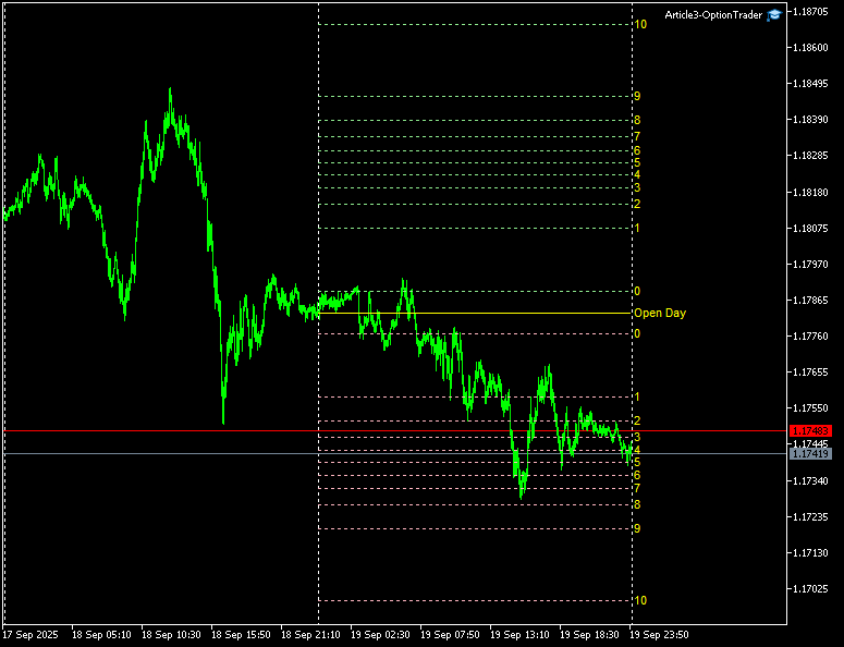
Fig. 2 Visualization of option levels

Complex option strategies

Now let's add some new strategies to our list of option structures:

// ---------------------------------------------------------------------
//  Option construction:
// ---------------------------------------------------------------------
enum ENUM_OPTION_CONSTRUCTION
{
  ENUM_OPTION_CONSTRUCTION_STRADDLE_LONG = 5,                         // Long STRADDLE
  ENUM_OPTION_CONSTRUCTION_STRADDLE_SHORT = 6,                        // Short STRADDLE
  ENUM_OPTION_CONSTRUCTION_STRANGLE_LONG = 7,                         // Long STRANGLE
  ENUM_OPTION_CONSTRUCTION_STRANGLE_SHORT = 8,                        // Short STRANGLE
};
// --------------------------------------------------------------------

Let's examine the purpose and conditions for using the new strategies listed above.

Buying a straddle — Long STRADDLE

• Meaning: the simultaneous buying of call and put options with the same strike prices;
• Condition for use: if there is confidence that the price of the underlying asset will rise or fall beyond the historical volatility (HV) range, but there are no assumptions about the direction;
• Profit: unlimited;
• Risk: the premium paid for two options (none in the emulation) + the loss incurred when rebalancing the option strategy.

The relationship between the delta value of the Delta option structure and the relative change in DPrice is shown in Fig. 3. This relationship arises when we buy two options with the same strike prices — Long Put and Long Call. The table to the left of the chart lists the DPrice values (x in the table), at which the option structure is rebalanced.

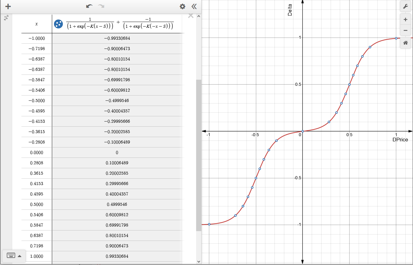
Fig. 3. Relationship between the Delta value and the relative change in DPrice (x — as shown in the table) for the emulated Long STRADDLE option strategy. S = 0.5, K = 10. The delta range is divided into ten equal parts

An illustrative graph showing the relationship between PnL (Profit/Loss) and the relative price change is shown in Fig. 4. It is important to understand that this chart is a theoretical representation based on the average historical volatility (HV) of the underlying asset price. Risk depends largely on the number of rebalancings of the option strategy — each rebalancing adds to the total PnL. This is the main difference between an emulated option and a real one.

The chart shows that maximum profit is achieved when the price of the underlying asset moves outside the HV volatility range (or, at the very least, does not fluctuate frequently between the option levels) — the areas highlighted in green in the figure illustrate this.

The left side of the DPrice axis (DPrice < 0) corresponds to a decline in the price of the underlying asset relative to the strike price — it is marked by an arrow pointing to the left labeled "Long Put working area, Long Call = 0" (the Long Put option's working area). In this region, the delta of Long Call option is zero; that is, it has no effect on the simulation of the aggregate option position.

The right side of the DPrice axis (DPrice > 0) corresponds to an increase in the price of the underlying asset relative to the strike price — it is marked by an arrow pointing to the right labeled "Long Call working area, Long Put = 0" (the Long Call option's working area). In this region, the delta of Long Put option is zero; that is, it has no effect on the simulation of the aggregate option position.

The chart also shows: profit (Profit), loss (Loss), and the strike price (Strike).

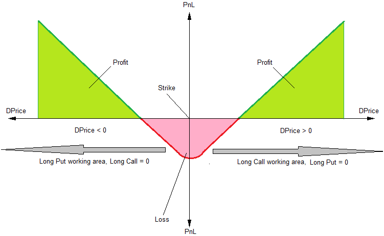
Fig. 4: Relationship between the "PnL" (profit/loss) value and the relative change in price (DPrice) for a simulated Long STRADDLE option strategy.

An example of how Long Straddle option strategy works is shown in Fig. 5. In this case, the option structure was held until expiration. Since the price fluctuated within the volatility range and had almost returned to the opening price by the end of the day, a small loss was incurred.

The chart also shows that around 3:00 p.m., the price of the underlying asset reached the seventh emulation level, making it possible to exercise the options early and fix a profit. Unlike with real options, there would be no liquidity issues.

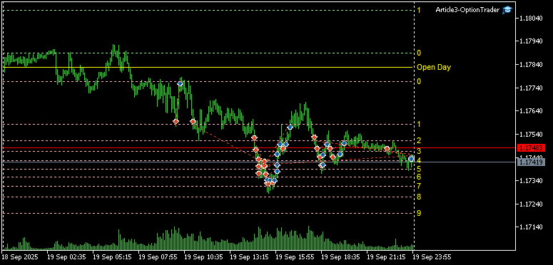
Fig. 5. Long Straddle option strategy

Selling a straddle — Short STRADDLE

• Meaning: The simultaneous sale of call and put options with the same strike prices;
• Condition for use: If you are confident that the price of the underlying asset remains within the average range of its historical volatility (HV), and the direction of the price movement is irrelevant;
• Profit: The premium paid by the buyer for the two options (not applicable in emulation) + the profit accumulated when the price fluctuates within the range (applicable only in emulation);
• Risk: Unlimited.

The relationship between the Delta option structure and the relative change in DPrice is shown in Fig. 6. This relationship arises when selling two options with the same strike prices — selling a put and a call. The table to the left of the graph lists the DPrice values (x in the table), at which the option structure is rebalanced.

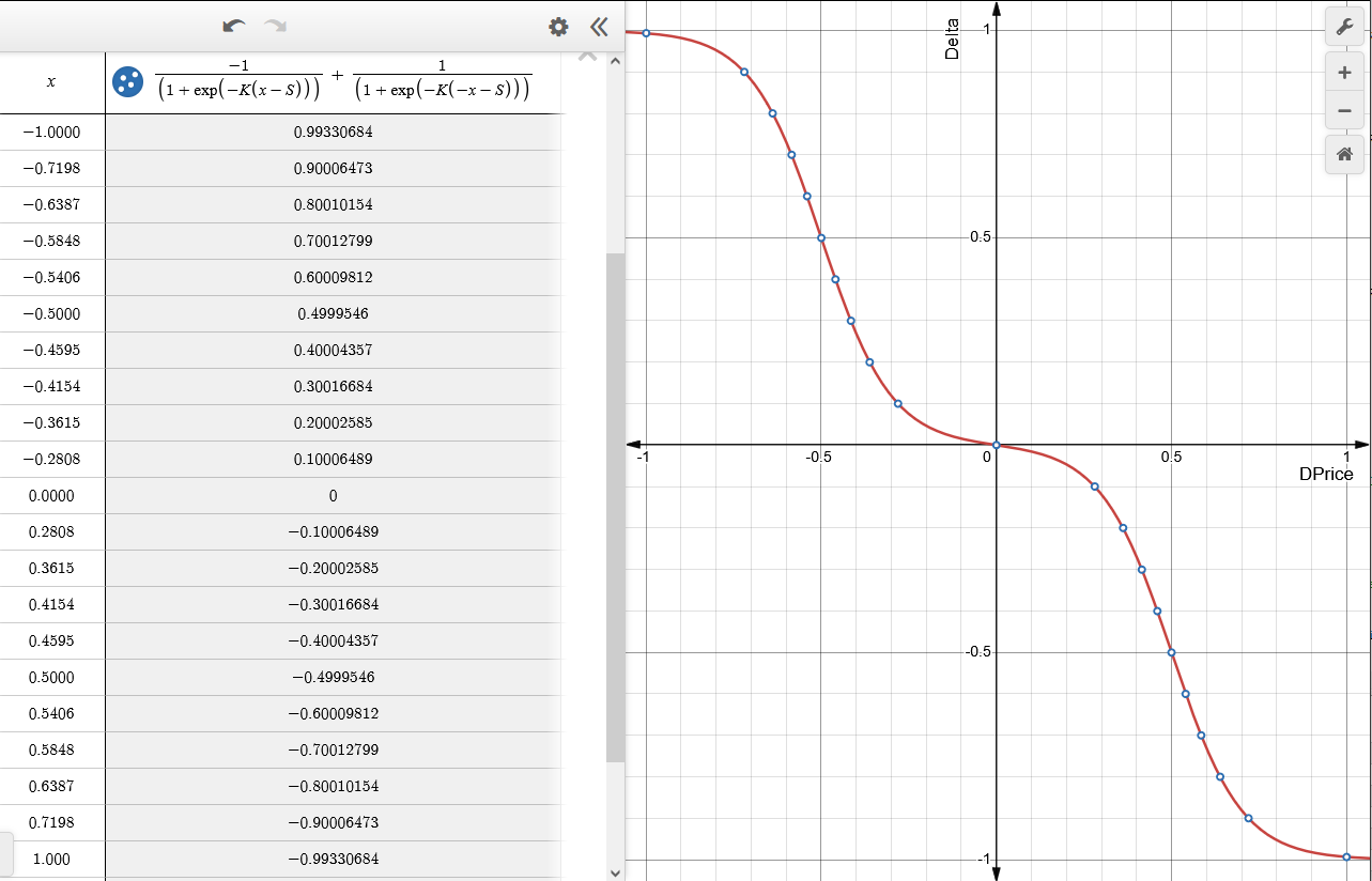
Fig. 6. Relationship between the Delta value and the relative change in price DPrice (x — as shown in the table) for the emulated Short STRADDLE option structure. S = 0.5, K = 10. The delta range is divided into ten equal parts

Fig. 7 shows an approximate graph illustrating the relationship between PnL (profit/loss) and the relative price change. It is important to understand that this chart is a theoretical representation based on the average historical volatility (HV) of the underlying asset's price. This is the main difference between a simulated option and a real one.

The chart shows that a profit is realized if the price of the underlying asset remains within the historical volatility (HV) range — shaded in green in the figure. The greater the price fluctuations between the option levels, the higher the profit at expiration (however, to maximize profit, the price should return as close as possible to the strike price). The direction of the fluctuations relative to the strike price is irrelevant — we end up with an almost ideal setup for range trading.

If the price of the underlying asset moves outside the historical volatility (HV) range and remains there until expiration, we will incur a loss. The farther the price moves beyond that range, the greater the loss. In theory, the risk is unlimited. In reality, we can always close our positions and stop the EA from running. There are more complex option structures that automatically reduce risk to an acceptable level and have virtually no impact on profits. More on this in the next article.

The left side of the DPrice axis (DPrice < 0) corresponds to a decline in the price of the underlying asset relative to the strike price — it is marked by an arrow pointing to the left labeled "Short Put working area, Short Call = 0" (Short Put option working area). In this region, the delta of the Short Call option is zero, meaning it has no effect on the simulation of the aggregate option position.

The right side of the DPrice axis (DPrice > 0) corresponds to an increase in the price of the underlying asset relative to the strike price — it is indicated by an arrow pointing to the right labeled "Short Call working area, Short Put = 0" (Short Call option working area). In this region, the delta of the Short Put option is zero; that is, it has no effect on the simulation of the aggregate option position.

The chart also shows: profit (Profit), loss (Loss), and the strike price (Strike).

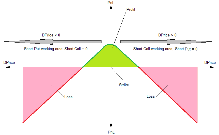
Fig. 7. Relationship between the PnL (profit/loss) value and the relative change in price (DPrice) for the simulated Short STRADDLE option strategy

An example of how the Short Straddle option strategy works is shown in Fig. 8. The highest level reached for intraday rebalancing of the option position was nine. It is clear to see how we generate profit with every fluctuation in the price of the underlying asset between the option levels. By the end of the day, before expiration, all positions had been closed — the price had returned to zero. In this case, our forecast that the price would remain within a certain range proved to be entirely accurate. Obviously, this is not always the case.

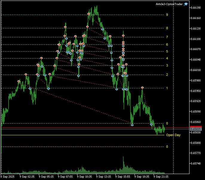
Fig. 8. Short Straddle option strategy

Buying a strangle — Long STRANGLE

• Meaning: The simultaneous buying of call and put options with different strike prices that fall within the historical volatility (HV) range;
• Condition for use: If you are confident that the price of the underlying asset will change significantly, but have no idea which direction it will take;
• Profit: unlimited;
• Risk: the premium paid for two options (none in the emulation) + the loss incurred when rebalancing the option strategy.

The difference from a Long Straddle is that this strategy uses two strike prices — one for the negative region of DPrice and one for the positive region. Between strikes, the position is zero; therefore, the current PnL in this range remains unchanged.

An approximate graph showing the relationship between PnL (Profit/Loss) and the relative price change is shown in Fig. 9. It is important to understand that this chart is a theoretical representation based on the average historical volatility (HV) of the underlying asset's price. Risk depends largely on the number of rebalancings of the option strategy — each rebalancing adds to the total PnL. This is the main difference between a simulated option and a real one.

The left side of the DPrice axis (DPrice < 0) corresponds to a decline in the price of the underlying asset relative to the Strike1 strike price — it is marked by an arrow pointing to the left labeled "Long Put working area, Long Call = 0" (the Long Put option's working area). In this region, the delta of Long Call option is zero; that is, it has no effect on the simulation of the aggregate option position.

The right side of the DPrice axis (DPrice > 0) corresponds to an increase in the price of the underlying asset relative to the Strike2 strike price — it is marked by an arrow pointing to the right with the label "Long Call working area, Long Put = 0" (the Long Call option's working area). In this region, the delta of Long Put option is zero; that is, it has no effect on the simulation of the aggregate option position.

The chart shows that maximum profit is achieved when the price of the underlying asset moves outside the HV volatility range (or, at the very least, does not fluctuate frequently between the option strike prices) — the areas highlighted in green in the figure illustrate this. Price fluctuations between strike prices have no effect on profit or loss, since the delta of both options is zero in this range.

The chart also shows: profit (Profit) and loss (Loss) zones, as well as the strike prices (Strike1 and Strike2).

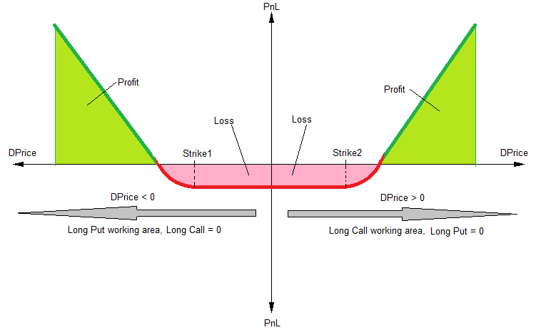
Fig. 9. Relationship between the PnL (profit/loss) value and the relative change in price (DPrice) for the simulated Long STRANGLE option strategy

An example of how the Long Strangle option strategy works is shown in Fig. 10. The non-linear distribution of emulation levels and the option position rebalancing trades are visible. The levels of Strike1 and Strike2 correspond to a relative price change (DPrice) equal to 0.1 times the historical volatility (HV) for the current day.

This value is set in the EA's external parameters using the variable shown below (it can range from 0.01 to 0.10):

input double StrangleKoeffStrike = 0.08; // Strangle Koeff for Strike (0.01...0.10)

In this case, the price of the underlying asset rose during the first half of the day and reached the eighth emulation level. Losses accumulated during the pullbacks, but as of the time this screenshot was taken, the position is showing a decent profit (even after accounting for closed losing trades). This suggests the possibility of early expiration — we will add this feature to the EA in the future. We will also automate early expiration by setting an expiration level.

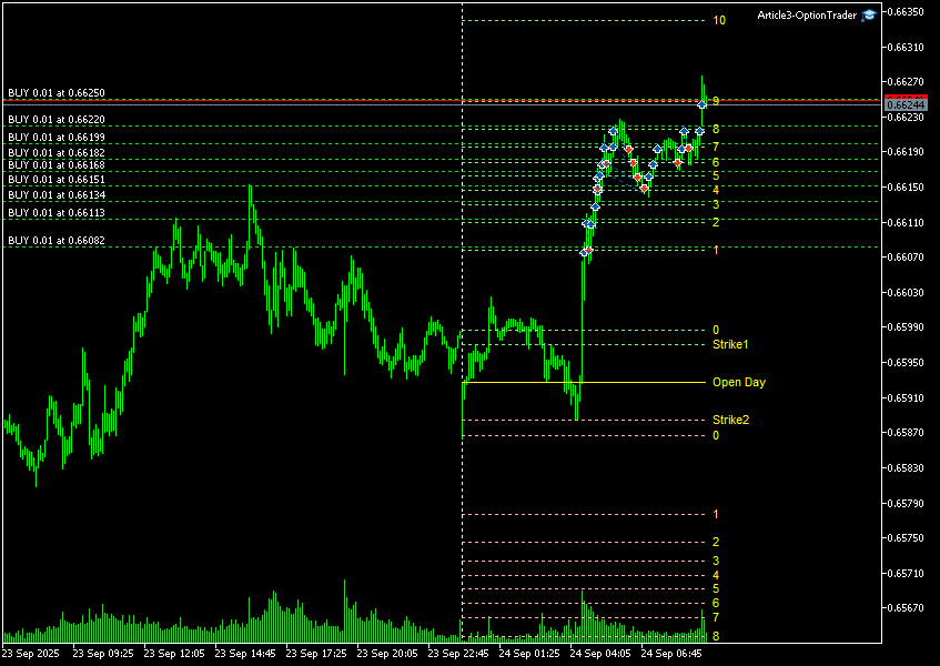
Fig. 10: Long Strangle option strategy

Selling a strangle — Short STRANGLE

• Meaning: The simultaneous sale of call and put options with different strike prices that fall within the historical volatility (HV) range
• Condition for use: If you are confident that the price of the underlying asset will remain within a wide range, and its direction is irrelevant
• Profit: the premium paid by the buyer for the two options (which is not paid in a simulated scenario) + the profit accumulated as the price fluctuates within a wide range
• Risk: unlimited

The difference from the Short Straddle is that this strategy uses two strike prices — one for the negative region of DPrice and one for the positive region. Between strikes, the position is zero; therefore, the current PnL in this range remains unchanged.

A sample graph showing the relationship between PnL (profit/loss) and the relative price change is shown in Fig. 11. It is important to understand that this chart is a theoretical representation based on the average historical volatility (HV) of the underlying asset's price. This is the main difference between a simulated option and a real one.

The chart shows that a profit is generated if the price of the underlying asset remains within the historical volatility (HV) range — shaded in green in the figure. The greater the price fluctuations between the option levels, the higher the profit at expiration (however, to maximize profit, the price should return as close as possible to the strike price). The direction of the fluctuations relative to the strike price is irrelevant — we end up with an almost ideal setup for range trading.

If the price of the underlying asset moves outside the historical volatility (HV) range and remains there until expiration, we will incur a loss. The farther the price moves beyond that range, the greater the loss. In theory, the risk is unlimited. In reality, we can always close our positions and stop the EA from running. There are more complex option structures that automatically reduce risk to an acceptable level and have virtually no impact on profits. More on this in the next article.

The left side of the DPrice axis (DPrice < 0) corresponds to a decline in the price of the underlying asset relative to the strike price — it is marked by an arrow pointing to the left labeled "Short Put working area, Short Call = 0" (Short Put option working area). In this region, the delta of the Short Call option is zero, meaning it has no effect on the simulation of the aggregate option position.

The right side of the DPrice axis (DPrice > 0) corresponds to an increase in the price of the underlying asset relative to the strike price — it is indicated by an arrow pointing to the right labeled "Short Call working area, Short Put = 0" (Short Call option working area). In this region, the delta of the Short Put option is zero; that is, it has no effect on the simulation of the aggregate option position.

The chart also shows: profit (Profit) and loss (Loss) zones, as well as the strike prices (Strike1 and Strike2).

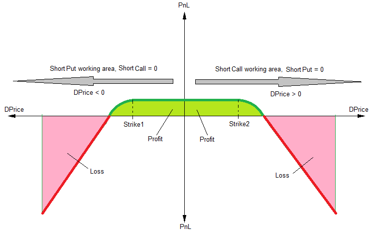
Fig. 11. Relationship between the PnL (profit/loss) value and the relative change in price (DPrice) for the simulated Short STRADDLE option strategy

An example of the Short Strangle option strategy is shown in Fig. 12. The levels of Strike1 and Strike2 correspond to a relative price change (DPrice) equal to 0.08 of the historical volatility (HV) for the current day. The chart shows that during the first half of the day, the price of the underlying asset fluctuated above the opening price — between the strike price and the fourth rebalancing level. As a result, some profit was generated.

At around 3:30 p.m. Moscow Time, the price of the underlying asset reversed downward and fluctuated several times between the first and fifth rebalancing levels — this generated some additional profit. At this point, we can already execute the options early to lock in the profits. Generally, the final decision always rests with the trader.

As we can see, for this options strategy, the direction of the underlying asset’s price movement is irrelevant — the key is that its price remains within the historical volatility (HV) range. This is true for a normal distribution of price increments, but in reality, price spikes in a single direction are possible. In this situation, either more complex option strategies or early closure of the position can help.

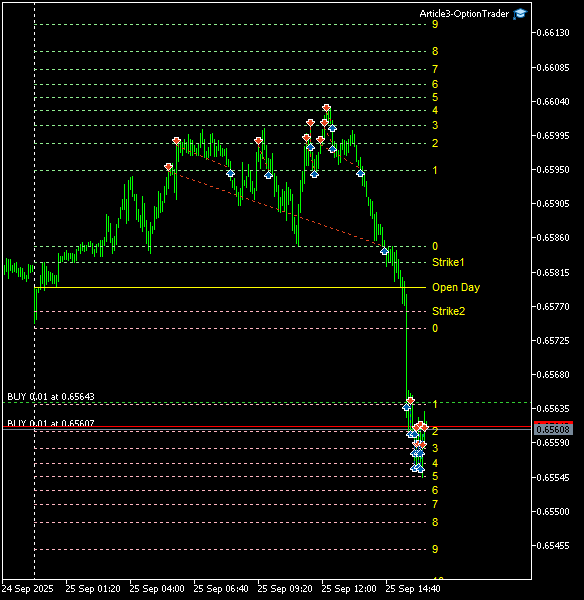
Fig. 12. Short Strangle option strategy

Implementing Long Straddle on MQL5

The StraddleLongOptionConstruction class, which creates an option structure, is derived from the TOptionConstructionBase base class (see the description in the previous article,“Trading Options Without Options (Part 2): Use in Real Trading”). The constructor parameters are the number of option levels (int _levels_number) during emulation and the maximum error (double _tolerance) when calculating prices corresponding to delta values for level visualization.

The StraddleLongOptionConstruction::CreateOptionConstruction(...) method creates two objects — one of OptionLongPut type and one of OptionLongCall type — and adds them to the CList list, from which the base class of the option construction, TOptionConstructionBase, is derived.

// =====================================================================
//  'Straddle Long' type option construction class:
// =====================================================================
class StraddleLongOptionConstruction : public TOptionConstructionBase
{
public:
  // ---------------------------------------------------------------------
  //  Constructor:
  // ---------------------------------------------------------------------
  StraddleLongOptionConstruction(const int _levels_number = 10, const double _tolerance = 0.00001)
  :
  TOptionConstructionBase(ENUM_OPTION_CONSTRUCTION_STRADDLE_LONG, _levels_number, _tolerance)
  {
  }
  // ---------------------------------------------------------------------
  //  Create option construction:
  // ---------------------------------------------------------------------
  void  CreateOptionConstruction(const double _k, const double _s, const int _digits) override
  {
    this.Add(new OptionLongPut(_k, _s, _digits));
    this.Add(new OptionLongCall(_k, _s, _digits));
  }

... the remaining part of the code is in the file "OptionEmulatorA3.mqh" ...

};

// ---------------------------------------------------------------------

The rest of the class methods are described in the previous article and earlier in this article.

Implementing Short Straddle on MQL5

The StraddleShortOptionConstruction class, which creates an option structure, is derived from the TOptionConstructionBase base class (see the description in the previous article). The constructor parameters are the number of option levels (int _levels_number) during emulation and the maximum error (double _tolerance) when calculating prices corresponding to delta values for level visualization.

The StraddleShortOptionConstruction::CreateOptionConstruction(...) method creates two objects — one of OptionShortPut type and one of OptionShortCall type — and adds them to CList, from which the base class of the option construction, TOptionConstructionBase, is derived.

// =====================================================================
//  Straddle Short type option construction class:
// =====================================================================
class StraddleShortOptionConstruction : public TOptionConstructionBase
{
public:
  // ---------------------------------------------------------------------
  //  Constructor:
  // ---------------------------------------------------------------------
  StraddleShortOptionConstruction(const int _levels_number = 10, const double _tolerance = 0.00001)
  :
  TOptionConstructionBase(ENUM_OPTION_CONSTRUCTION_STRADDLE_SHORT, _levels_number, _tolerance)
  {
  }
  // ---------------------------------------------------------------------
  //  Create option construction:
  // ---------------------------------------------------------------------
  void  CreateOptionConstruction(const double _k, const double _s, const int _digits) override
  {
    this.Add(new OptionShortPut(_k, _s, _digits));
    this.Add(new OptionShortCall(_k, _s, _digits));
  }

... the remaining part of the code is in the file "OptionEmulatorA3.mqh" ...

};

// ---------------------------------------------------------------------

The rest of the class methods are described in the previous article and earlier in this article.

Implementing Long Strangle on MQL5

The StrangleLongOptionConstruction class, which creates an option structure, is derived from the TOptionConstructionBase base class (see the description in the previous article). The constructor parameters are the number of option levels (int _levels_number) during emulation and the maximum error (double _tolerance) when calculating prices corresponding to delta values for level visualization.

The StrangleLongOptionConstruction::CreateOptionConstruction(...) method creates two objects — one of OptionLongPut type and one of OptionLongCall type — and adds them to the CList, from which the base class of the option construction, TOptionConstructionBase, is derived.

// =====================================================================
//  Strangle Long type option construction class:
// =====================================================================
class StrangleLongOptionConstruction : public TOptionConstructionBase
{
public:
  // ---------------------------------------------------------------------
  //  Constructor:
  // ---------------------------------------------------------------------
  StrangleLongOptionConstruction(const int _levels_number = 10, const double _tolerance = 0.00001)
  :
  TOptionConstructionBase(ENUM_OPTION_CONSTRUCTION_STRANGLE_LONG, _levels_number, _tolerance)
  {
  }
  // ---------------------------------------------------------------------
  //  Create option construction:
  // ---------------------------------------------------------------------
  void  CreateOptionConstruction(const double _k, const double _s, const int _digits) override
  {
    this.Add(new OptionLongPut(_k, _s, _digits));
    this.Add(new OptionLongCall(_k, _s, _digits));
  }

... the remaining part of the code is in the file "OptionEmulatorA3.mqh" ...

};
// ---------------------------------------------------------------------

This option strategy differs from Long Straddle in that different strike prices — Strike1 and Strike2 — are set for Long Put and Long Call options. The rest of the class methods are described in the previous article and earlier in this article.

Implementing Short Strangle on MQL5

The StrangleShortOptionConstruction class, which creates an option structure, is derived from the base class TOptionConstructionBase (see the description in the previous article). The constructor parameters are the number of option levels (int _levels_number) during emulation and the maximum error (double _tolerance) when calculating prices corresponding to delta values for level visualization.

The StrangleShortOptionConstruction::CreateOptionConstruction(...) method creates two objects—one of type OptionShortPut and one of type OptionShortCall —and adds them to the CList, from which the base class of the option construction, TOptionConstructionBase, is derived.

// =====================================================================
//  Strangle Short type option construction class:
// =====================================================================
class StrangleShortOptionConstruction : public TOptionConstructionBase
{
public:
  // ---------------------------------------------------------------------
  //  Constructor:
  // ---------------------------------------------------------------------
  StrangleShortOptionConstruction(const int _levels_number = 10, const double _tolerance = 0.00001)
  :
  TOptionConstructionBase(ENUM_OPTION_CONSTRUCTION_STRANGLE_SHORT, _levels_number, _tolerance)
  {
  }
  // ---------------------------------------------------------------------
  //  Create option construction:
  // ---------------------------------------------------------------------
  void  CreateOptionConstruction(const double _k, const double _s, const int _digits) override
  {
    this.Add(new OptionShortPut(_k, _s, _digits));
    this.Add(new OptionShortCall(_k, _s, _digits));
  }
... the remaining part of the code is in the file "OptionEmulatorA3.mqh" ...

};

// --------------------------------------------------------------------

The difference between this option strategy and Short Straddle is that different strike prices — Strike1 and Strike2 — are set for the Short Put and Short Call options. The rest of the class methods are described in the previous article in this series and earlier in this article.

Conclusion

As we can see, implementing option structures using an object-oriented approach is quite simple and easy to understand. All implementation details are encapsulated in the base classes. That said, the complexity of the option structure (in other words, the number of items in the CList) is limited only by the user's imagination and the computer's resources.

The two-option structures described in the article are used quite widely in trading — in particular, on the MOEX exchange. However, there are also more complex four-option strategies that allow reducing the risks associated with the options you have bought and lock in profits on the options you have sold — these will be discussed in the fourth article of this series.

We are also upgrading our EA by adding level-triggered expiration — this will allow us to automatically lock in profits for strategies that involve buying options.

The following table lists all the files attached to the article:

File name	Description
Article3-OpionTrader.mq5	The code for the EA that trades the option strategies described in the article using option emulation
CheckNewBar.mq5	The class code to check for the appearance of a new bar on the MetaTrader 5 terminal chart
OptionEmulatorA3.mq5	The code of the classes for emulating the options and option structures described in the article
PriceLevelsA3.mq5	The class code for displaying option levels on the MetaTrader 5 terminal chart