Reimagining Classic Strategies (Part 16): Double Bollinger Band Breakouts

MetaTrader 5 — Examples | 2 October 2025, 08:05

373

Financial markets are not just static, fixed machines that exist in discrete states. Rather, financial markets are living, breathing, and intelligent systems that react to information. They are constantly shifting and never settle on any state permanently, yet most trading strategies treat them as though they do.

Most trading strategies generally classify the market as being either trending or range-bound, and then they suggest steps to follow, depending on the identified state of the market. This article aims to illustrate to the reader that this view of the market is just too simple to be practical. If we want strategies that can actually keep up with ever-changing markets, markets that can at times even act in adversarial modes, then we need tools that accept financial markets for what they are: a constantly evolving and only partially observable system.

That’s where trading strategies such as the double Bollinger Band system come in. It is an extension of the classical Bollinger Band system, and it is widely attributed to having originated from institutional traders. It is adapted to capture changing market conditions smoothly. The backtested results we will demonstrate shortly, will back our remarks. Most Bollinger Band trading strategies are limited to textbook rules and tend to assume that you will be working under favorable market conditions. They tell you to trade breakouts or to trade fades, but they do not capture the messy reality of how markets actually behave, constantly alternating between favorable and unfavorable states.

In our methodology, we have implemented a well known variation of the classical Bollinger Band strategy that is widely known by most traders in our community. This version of the strategy set profitability benchmarks for the Double Bollinger Bands to outperform. As we shall soon discuss, when we tested the standard Bollinger Band breakout, we actually lost money.

Both strategies were tested over the same five-year historical period, running from January 2020 through 2025. We tried our best to ensure that both strategies relied on identical parameters wherever we found it possible to do so. The classical strategy lost money consistently, while the double Bollinger Band system outperformed it remarkably, with fixed parameters such as the period of the Bollinger Bands, and the lot size used. We will go over these results in more detail. But for now, I will briefly summarize our key findings.

The classical strategy produced a gross loss of -$169 over five years, while the double Bollinger Band system generated a gross profit of $228 under the same conditions and using fixed parameters wherever possible. For fairness, all trades were opened at minimum lot size, and each strategy was limited to one open trade at a time. Additionally, the classical strategy also produced a negative Sharpe ratio of –0.53, whereas the improved version achieved a positive Sharpe ratio of 0.5. This marks a clear improvement in profitability and stability.

Looking at accuracy, the classical strategy produced 46% winning trades over five years—not impressive. The double Bollinger Band system, however, achieved 56% winning trades, a 21% improvement in accuracy. Even more striking, the asymmetric manner in which we changed the distribution of profits and losses. The solution we present to the reader increased the gross profits of the back test by 70%, but only increased gross losses by 17%. This asymmetric effect—profits growing faster than losses—shows how appropriately the double Bollinger Band system reshapes trade distribution into a more desirable form.

Finally, considering the changes in profit factor, the original strategy produced a factor of 0.82, meaning it lost capital over time. The double Bollinger Band system produced a factor of 1.2, a key indication of capital growth, which represents a 50% improvement in profit factor.

Taken together, these results suggest that the double Bollinger Band system is not merely an upgrade to the original but a paradigm shift. It represents a new family of strategies that share ancestry with the classical approach but fundamentally change its outcome. The system turned a losing strategy into a winning one, dramatically improved profitability, and did so while maintaining remarkable control over risk.

Most importantly, it achieved these improvements without adding unnecessary complexity. The double Bollinger Band system is still easy to learn, implement, and interpret, yet it offers far greater benefits. This excites me most because in the future, if we choose to add complexity—through machine learning models to optimize entries and exits or even feedback controllers to adapt to dominant patterns—we can be confident the effort will be worthwhile and that the underlying strategy is profitable.

Even without such additions, the double Bollinger Band system already provides simplicity with an edge—a highly desirable feature for any trading application. Let us get started.

Overview of The Classical Trading Strategy

We begin by first applying the classical Bollinger Bands indicator onto our chart as we normally would. For this discussion, we have selected the EURUSD pair, and we will be analyzing it from the daily time frame. Therefore, in Figure 1 below, we have set the Bollinger Bands to use a period of 20 daily candles. We will mark our upper and lower bands 2 standard deviations from the middle band, as this is the classical setup.

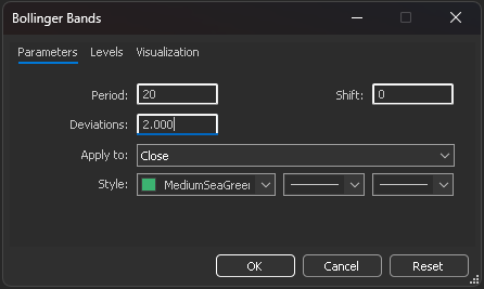
Figure 1: Applying our Bollinger Bands indicator to the EURUSD pair with classical input settings

The classical version of the trading strategy is straightforward. Whenever price levels break above the uppermost band, we will pick short entries. And the opposite is true when price levels break below the lowest band, we will enter long positions. The reasoning behind the classical Bollinger Band strategy is that markets move in mean-reverting cycles. Therefore, breakouts beyond either extreme band level are expected to be followed up by price action that returns price levels to the middle band.

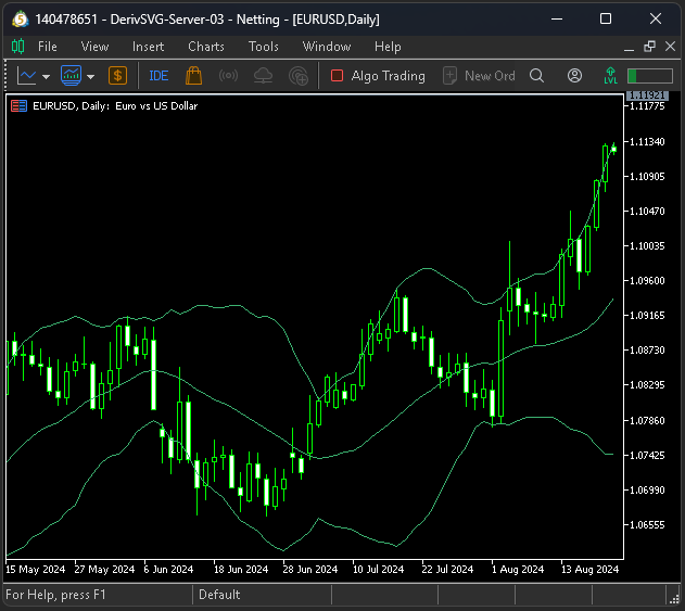
Figure 2: Visualizing the classical version of the Bollinger Band strategy

As with any trading strategy, there are inherent limitations associated with the trading rules we have defined for the classical setup. It is widely known that such trading strategies are susceptible to false breakouts. Simply put, market conditions may lethargically drift enough to trigger our entry signals before violently changing course and reverting to their original trajectory. Such trading conditions will consistently drain any investor's equity.

Figure 3 below may help the reader visualize the weakness of the strategy we are highlighting. In the image, we can see 2 sell setups that have been correctly identified using the rules we have defined earlier. However, as we can see, only one of the trades produced the expected outcome. In the first trade, bounded by the green box, price levels reverted to mid-band after they momentarily broke above the upper band. However, it then appeared to repeat the same pattern in the time bounded by the candles in the red box, but this was a false breakout. Price levels continued to rally and did not revert to mid-band as anticipated by the classical strategy.

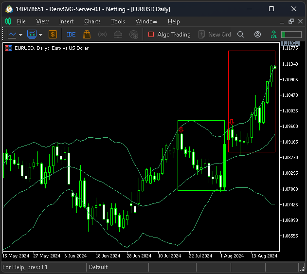
Figure 3: Visualizing the limitations of the classical Bollinger Band strategy

Getting Started In MQL5

As with most of our trading applications, we begin by defining system constants. These definitions are the cornerstone of our tests because they keep as many parameters fixed as possible across both experiments. Important parameters , the period of the Bollinger Bands, the shifts, indicator lookbacks, timeframes, and the standard deviations used for the bands, must remain fixed because they greatly change the behavior of the strategy.

//+------------------------------------------------------------------+
//|                                                DBB Benchmark.mq5 |
//|                                               Gamuchirai Ndawana |
//|                    https://www.mql5.com/en/users/gamuchiraindawa |
//+------------------------------------------------------------------+
#property copyright "Gamuchirai Ndawana"
#property link      "https://www.mql5.com/en/users/gamuchiraindawa"
#property version   "1.00"

//+------------------------------------------------------------------+
//| System definitions                                               |
//+------------------------------------------------------------------+
#define BB_PERIOD   20
#define BB_SHIFT    0
#define ATR_PERIOD  14
#define ATR_PADDING 2
#define BB_SD_1     2
#define BB_SD_2     1
#define TF_1        PERIOD_D1

After constants, we define global variables. Most global variables relate to the technical indicators we rely on and the stop-loss sizing we will use.

//+------------------------------------------------------------------+
//| Global variables                                                 |
//+------------------------------------------------------------------+
int    bb_handler,bb_handler_2,atr_handler;
double bb_reading_u[],bb_reading_m[],bb_reading_l[],bb_reading_u_2[],bb_reading_m_2[],bb_reading_l_2[],atr_reading[];
double padding,close;

Afterward, we will import the libraries needed for trading and for recording trade information such as bid and ask prices. Libraries play an important role in almost any application development process because we rarely write all code from scratch.

//+------------------------------------------------------------------+
//| Library                                                          |
//+------------------------------------------------------------------+
#include <Trade\Trade.mqh>
#include <VolatilityDoctor\Trade\TradeInfo.mqh>

CTrade    Trade;
TradeInfo *TradeInfoHandler;

When the application loads for the first time, we initialize the global variables: empty data structures and a new instance of our custom trade-information class.

//+------------------------------------------------------------------+
//| Expert initialization function                                   |
//+------------------------------------------------------------------+
int OnInit()
  {
//--- Setup our technical indicators
   bb_handler       = iBands(Symbol(),TF_1,BB_PERIOD,BB_SHIFT,BB_SD_1,PRICE_CLOSE);
   bb_handler_2     = iBands(Symbol(),TF_1,BB_PERIOD,BB_SHIFT,BB_SD_2,PRICE_CLOSE);
   atr_handler      = iATR(Symbol(),TF_1,ATR_PERIOD);
   TradeInfoHandler = new TradeInfo(Symbol(),TF_1);
//---
   return(INIT_SUCCEEDED);
  }

If the application should no longer be in use, we must remember to free memory resources that were previously allocated to handlers we defined earlier.

//+------------------------------------------------------------------+
//| Expert deinitialization function                                 |
//+------------------------------------------------------------------+
void OnDeinit(const int reason)
  {
//--- Release the indicators we are no longer using
   IndicatorRelease(bb_handler);
   IndicatorRelease(bb_handler_2);
   IndicatorRelease(atr_handler);
  }

In the classical setup of the strategy, entry logic is simple and easy to interpret. If the Bollinger Band high is broken by the closing price, we sell; if the Bollinger Band low is broken by the closing price and we have no open positions, we buy.

//+------------------------------------------------------------------+
//| Expert tick function                                             |
//+------------------------------------------------------------------+
void OnTick()
  {
//--- Keep track of time
   static datetime timestamp;
   datetime current_time = iTime(Symbol(),TF_1,0);

   if(timestamp != current_time)
     {
      //--- Update indicator readings
      CopyBuffer(bb_handler,0,0,1,bb_reading_m);
      CopyBuffer(bb_handler,1,0,1,bb_reading_u);
      CopyBuffer(bb_handler,2,0,1,bb_reading_l);
      CopyBuffer(bb_handler_2,0,0,1,bb_reading_m_2);
      CopyBuffer(bb_handler_2,1,0,1,bb_reading_u_2);
      CopyBuffer(bb_handler_2,2,0,1,bb_reading_l_2);
      CopyBuffer(atr_handler,0,0,1,atr_reading);

      //--- Get updated market readings
      close = iClose(Symbol(),TF_1,0);
      padding = atr_reading[0] * 2;

      //--- If we have no open positions
      if(PositionsTotal() == 0)
        {
         if(close > bb_reading_u[0])
            Trade.Sell(TradeInfoHandler.MinVolume(),Symbol(),TradeInfoHandler.GetBid(),TradeInfoHandler.GetAsk()+padding,TradeInfoHandler.GetAsk()-padding);

         else
            if(close < bb_reading_l[0])
               Trade.Buy(TradeInfoHandler.MinVolume(),Symbol(),TradeInfoHandler.GetAsk(),TradeInfoHandler.GetBid()-padding,TradeInfoHandler.GetBid()+padding);
        }
     }
  }
//+------------------------------------------------------------------+

After the application has finished running, we undefine the system constants we built at the beginning—again, best practice for MQL5 code.

//+------------------------------------------------------------------+
//| Undefine system definitions                                      |
//+------------------------------------------------------------------+
#undef BB_PERIOD
#undef BB_SD_1
#undef BB_SD_2
#undef BB_SHIFT
#undef ATR_PADDING
#undef ATR_PERIOD
#undef TF_1
//+------------------------------------------------------------------+

When all pieces are combined, this is the control setup for our classical application.

//+------------------------------------------------------------------+
//|                                                DBB Benchmark.mq5 |
//|                                               Gamuchirai Ndawana |
//|                    https://www.mql5.com/en/users/gamuchiraindawa |
//+------------------------------------------------------------------+
#property copyright "Gamuchirai Ndawana"
#property link      "https://www.mql5.com/en/users/gamuchiraindawa"
#property version   "1.00"

//+------------------------------------------------------------------+
//| System definitions                                               |
//+------------------------------------------------------------------+
#define BB_PERIOD   20
#define BB_SHIFT    0
#define ATR_PERIOD  14
#define ATR_PADDING 2
#define BB_SD_1     2
#define BB_SD_2     1
#define TF_1        PERIOD_D1

//+------------------------------------------------------------------+
//| Global variables                                                 |
//+------------------------------------------------------------------+
int    bb_handler,bb_handler_2,atr_handler;
double bb_reading_u[],bb_reading_m[],bb_reading_l[],bb_reading_u_2[],bb_reading_m_2[],bb_reading_l_2[],atr_reading[];
double padding,close;

//+------------------------------------------------------------------+
//| Library                                                          |
//+------------------------------------------------------------------+
#include <Trade\Trade.mqh>
#include <VolatilityDoctor\Trade\TradeInfo.mqh>

CTrade    Trade;
TradeInfo *TradeInfoHandler;
//+------------------------------------------------------------------+
//| Expert initialization function                                   |
//+------------------------------------------------------------------+
int OnInit()
  {
//--- Setup our technical indicators
   bb_handler       = iBands(Symbol(),TF_1,BB_PERIOD,BB_SHIFT,BB_SD_1,PRICE_CLOSE);
   bb_handler_2     = iBands(Symbol(),TF_1,BB_PERIOD,BB_SHIFT,BB_SD_2,PRICE_CLOSE);
   atr_handler      = iATR(Symbol(),TF_1,ATR_PERIOD);
   TradeInfoHandler = new TradeInfo(Symbol(),TF_1);
//---
   return(INIT_SUCCEEDED);
  }
//+------------------------------------------------------------------+
//| Expert deinitialization function                                 |
//+------------------------------------------------------------------+
void OnDeinit(const int reason)
  {
//--- Release the indicators we are no longer using
   IndicatorRelease(bb_handler);
   IndicatorRelease(bb_handler_2);
   IndicatorRelease(atr_handler);
  }
//+------------------------------------------------------------------+
//| Expert tick function                                             |
//+------------------------------------------------------------------+
void OnTick()
  {
//--- Keep track of time
   static datetime timestamp;
   datetime current_time = iTime(Symbol(),TF_1,0);

   if(timestamp != current_time)
     {
      //--- Update indicator readings
      CopyBuffer(bb_handler,0,0,1,bb_reading_m);
      CopyBuffer(bb_handler,1,0,1,bb_reading_u);
      CopyBuffer(bb_handler,2,0,1,bb_reading_l);
      CopyBuffer(bb_handler_2,0,0,1,bb_reading_m_2);
      CopyBuffer(bb_handler_2,1,0,1,bb_reading_u_2);
      CopyBuffer(bb_handler_2,2,0,1,bb_reading_l_2);
      CopyBuffer(atr_handler,0,0,1,atr_reading);

      //--- Get updated market readings
      close = iClose(Symbol(),TF_1,0);
      padding = atr_reading[0] * 2;

      //--- If we have no open positions
      if(PositionsTotal() == 0)
        {
               if(close > bb_reading_u[0])
                  Trade.Sell(TradeInfoHandler.MinVolume(),Symbol(),TradeInfoHandler.GetBid(),TradeInfoHandler.GetAsk()+padding,TradeInfoHandler.GetAsk()-padding);

               else
                  if(close < bb_reading_l[0])
                     Trade.Buy(TradeInfoHandler.MinVolume(),Symbol(),TradeInfoHandler.GetAsk(),TradeInfoHandler.GetBid()-padding,TradeInfoHandler.GetBid()+padding);
        }
     }
  }
//+------------------------------------------------------------------+

//+------------------------------------------------------------------+
//| Undefine system definitions                                      |
//+------------------------------------------------------------------+
#undef BB_PERIOD
#undef BB_SD_1
#undef BB_SD_2
#undef BB_SHIFT
#undef ATR_PADDING
#undef ATR_PERIOD
#undef TF_1
//+------------------------------------------------------------------+

Now let us analyze the application’s performance over the five-year backtest. The total net profit is −169, which is not impressive. The Sharpe ratio is −0.53, and the percentage of profitable trades is below 50% at 46%. In short, this application performs worse than chance and is consistently unprofitable.

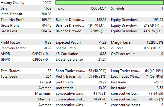
Figure 4: Visualizing the detailed statistics produced by the classical trading strategy

The equity curve for the classical strategy shows a persistent downtrend that grows stronger over time.

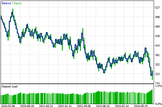
Figure 5: The classical version of the trading strategy produces a negative trend over time

Overview of The Revised Trading Strategy

The improvement is straightforward: instead of a single Bollinger Band system, we use two sets of bands. The inner band uses a smaller standard deviation, and the outer band uses a larger one. When the inner band is broken, we interpret that as a trend-following signal; when the outer (two-standard-deviation) band is broken, we interpret that as a mean-reversion signal. Concretely, if the inner-band is broken at the high, we buy (trend following); if the outer-band is broken at the high, we sell (mean reversion). The inverse of these rules holds true for the lower bands.

To realize this strategy, we only need to modify the entry rules; most of the code remains unchanged.

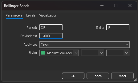
Figure 6: We will add a second filter, a tighter Bollinger Band standard deviation level, but we will keep the period fixed

We can visualize the revised version of the strategy using our MetaTrader 5 Terminal. Kindly note, you do not need to delete the first indicator we applied, or change to a new chart. Simply apply a second instance of the Bollinger Band indicator on the same chart you selected if you have been following along.

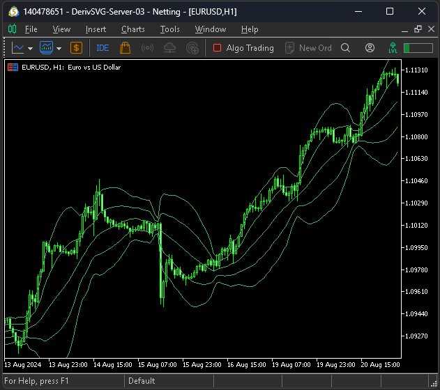
Figure 7: Visualizing the reimagined version of the classical Bollinger Band strategy

Implementing Our Improvements

We are now ready to implement the improvements of the double-Bollinger-band strategy.

//--- If we have no open positions
if(PositionsTotal() == 0)
      {
         //--- Is the close price above the highest band? Buy
         if(close > bb_reading_u[0])
            Trade.Buy(TradeInfoHandler.MinVolume(),Symbol(),TradeInfoHandler.GetAsk(),TradeInfoHandler.GetBid()-padding,TradeInfoHandler.GetBid()+padding);

         //--- Is the close price below the lowest band? Sell
         else
            if(close < bb_reading_l[0])
               Trade.Sell(TradeInfoHandler.MinVolume(),Symbol(),TradeInfoHandler.GetBid(),TradeInfoHandler.GetAsk()+padding,TradeInfoHandler.GetAsk()-padding);

            //--- Is the close price above the mid-high band? Sell
            else
               if((close < bb_reading_u[0]) && (close > bb_reading_l[0]) && (close > bb_reading_u_2[0]))
                  Trade.Sell(TradeInfoHandler.MinVolume(),Symbol(),TradeInfoHandler.GetBid(),TradeInfoHandler.GetAsk()+padding,TradeInfoHandler.GetAsk()-padding);

               //--- Is the close price below the mid-low band? Buy
               else
                  if((close < bb_reading_u[0]) && (close > bb_reading_l[0]) && (close < bb_reading_l_2[0]))
                     Trade.Buy(TradeInfoHandler.MinVolume(),Symbol(),TradeInfoHandler.GetAsk(),TradeInfoHandler.GetBid()-padding,TradeInfoHandler.GetBid()+padding);
      }

We will run the backtest over the same five-year window, spanning from January 2020 until March 2025.

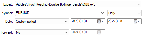
Figure 8: Testing the improved version of the double Bollinger Band trading strategy

As always, we use random delay settings with every take position on real ticks to better emulate real market latency and unpredictability.

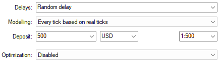
Figure 9: Select random delay settings for a reliable emulation of real market conditions

Examining the detailed statistics for the improved strategy, we see a clear change across the board. Total net profit becomes positive and nearly doubles in absolute terms compared with the classical system. Expected payoff rises, profit factor improves, and the percentage of profitable trades increases to a more attractive 56%. Often, improving a strategy reduces the number of trades while increasing profitability. In this case, however, both the total number of trades and the net profit have risen. That suggests the improved version uncovers additional signals that the original system was blind to.

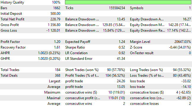
Figure 10: The revised trading strategy has materially improved the performance statistics of our trading application

Finally, the equity curve for the improved strategy has been completely transformed: the earlier negative trend is now a positive one, and the new equity curve is reaching higher peaks that the old curve could never have achieved, no matter how long it ran.

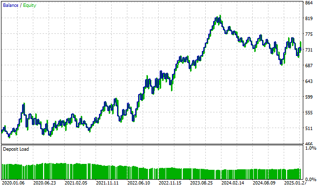
Figure 11: The equity curve produced by the revised trading strategy is finally profitable

Conclusion

After reading this article, the reader will see that classical trading strategies we think we understand may actually hold potential we have not yet realized.

The MQL5 API allows us to reimagine these strategies. With well-defined methods and other utilities, it can capture a wide variety of trading applications, even though the size of the API is fixed. Yes, the MQL5 API is growing every week with new updates, constantly being added to the MQL5 framework.

But even with just the core utilities, we can consistently create new applications capable of bridging the blind spots that classical strategies have. The MQL5 API gives us methods that reach broad and dynamic levels of utility—exactly what we need to build applications that are more aware of changes in market states, unlike their classical ancestors, which only viewed markets in static, binary terms.

File Name	File Description
DBB.mq5	The revised double Bollinger-Band trading strategy we implemented to improve our results.
DBB_Benchmark.mq5	The classical implementation of the Bollinger-Band strategy.

Attached files |

Download ZIP

DBB.mq5 (5.29 KB)

DBB_Benchmark.mq5 (4.47 KB)

Warning: All rights to these materials are reserved by MetaQuotes Ltd. Copying or reprinting of these materials in whole or in part is prohibited.

This article was written by a user of the site and reflects their personal views. MetaQuotes Ltd is not responsible for the accuracy of the information presented, nor for any consequences resulting from the use of the solutions, strategies or recommendations described.

Overview of The Classical Trading Strategy

Getting Started In MQL5

Overview of The Revised Trading Strategy

Implementing Our Improvements

Conclusion

Other articles by this author