Integrating MQL5 with data processing packages (Part 4): Big Data Handling

Introduction

Financial markets keep on evolving, traders are no longer dealing with just price charts and simple indicators—they're contending with a flood of data from every corner of the world. In this era of big data, successful trading isn’t just about strategy; it’s about how efficiently you can sift through mountains of information to find actionable insights. This article, the fourth in our series on integrating MQL5 with data processing tools, focuses on equipping you with the skills to handle massive datasets seamlessly. From real-time tick data to historical archives spanning decades, the ability to tame big data is quickly becoming the hallmark of a sophisticated trading system.

Imagine analyzing millions of data points to uncover subtle market trends or incorporating external datasets like social sentiment or economic indicators into your MQL5 trading environment. The possibilities are endless—but only if you have the right tools. In this piece, we’ll explore how to push MQL5 beyond its built-in capabilities by integrating it with advanced data processing libraries and big data solutions. Whether you're a seasoned trader aiming to refine your edge or a curious developer exploring the potential of financial technology, this guide promises to be a game-changer. Stay tuned to learn how you can turn overwhelming data into a decisive advantage.

Gather Historical Data

from datetime import datetime
import MetaTrader5 as mt5
import pandas as pd
import pytz

# Display data on the MetaTrader 5 package
print("MetaTrader5 package author: ", mt5.__author__)
print("MetaTrader5 package version: ", mt5.__version__)

# Configure pandas display options
pd.set_option('display.max_columns', 500)
pd.set_option('display.width', 1500)

# Establish connection to MetaTrader 5 terminal
if not mt5.initialize():
    print("initialize() failed, error code =", mt5.last_error())
    quit()

# Set time zone to UTC
timezone = pytz.timezone("Etc/UTC")
# Create 'datetime' objects in UTC time zone to avoid the implementation of a local time zone offset
utc_from = datetime(2024, 8, 6, tzinfo=timezone.utc)
utc_to = datetime.now(timezone)  # Set to the current date and time

# Get bars from BTC H1 (hourly timeframe) within the specified interval
rates = mt5.copy_rates_range("BTCUSD", mt5.TIMEFRAME_H1, utc_from, utc_to)

# Shut down connection to the MetaTrader 5 terminal
mt5.shutdown()

# Check if data was retrieved
if rates is None or len(rates) == 0:
    print("No data retrieved. Please check the symbol or date range.")
else:
    # Display each element of obtained data in a new line (for the first 10 entries)
    print("Display obtained data 'as is'")
    for rate in rates[:10]:
        print(rate)

    # Create DataFrame out of the obtained data
    rates_frame = pd.DataFrame(rates)
    # Convert time in seconds into the 'datetime' format
    rates_frame['time'] = pd.to_datetime(rates_frame['time'], unit='s')

    # Save the data to a CSV file
    filename = "BTC_H1.csv"
    rates_frame.to_csv(filename, index=False)
    print(f"\nData saved to file: {filename}")

To retrieve historical data, we first establish a connection to the MetaTrader 5 terminal using the `mt5.initialize()` function. This is essential because the Python package communicates directly with the running MetaTrader 5 platform. We configure the code to set the desired time range for data extraction by specifying the start and end dates. The `datetime` objects are created in the UTC time zone to ensure consistency across different time zones. The script then uses the `mt5.copy-rates-range()` function to request historical hourly data for the BTC/USD symbol, starting from August 6, 2024, up to the current date and time.

After disconnecting from the Meta Trader 5 terminal using `mt5.shutdown()` to avoid any further unnecessary connections. The retrieved data is initially displayed in its raw format to confirm successful data extraction. We then convert this data into a pandas Data Frame for easier manipulation and analysis. Additionally, the code converts the Unix timestamps into a readable datetime format, ensuring the data is well-structured and ready for further processing or analysis.

filename = "XAUUSD_H1_2nd.csv"
rates_frame.to_csv(filename, index=False)
print(f"\nData saved to file: {filename}")

Since my Operating System is Linux I have to save the received data into a file. But for those who are on Windows, you can simply retrieve the data with the following script:

from datetime import datetime
import MetaTrader5 as mt5
import pandas as pd
import pytz

# Display data on the MetaTrader 5 package
print("MetaTrader5 package author: ", mt5.__author__)
print("MetaTrader5 package version: ", mt5.__version__)

# Configure pandas display options
pd.set_option('display.max_columns', 500)
pd.set_option('display.width', 1500)

# Establish connection to MetaTrader 5 terminal
if not mt5.initialize():
    print("initialize() failed, error code =", mt5.last_error())
    quit()

# Set time zone to UTC
timezone = pytz.timezone("Etc/UTC")
# Create 'datetime' objects in UTC time zone to avoid the implementation of a local time zone offset
utc_from = datetime(2024, 8, 6, tzinfo=timezone.utc)
utc_to = datetime.now(timezone)  # Set to the current date and time

# Get bars from BTCUSD H1 (hourly timeframe) within the specified interval
rates = mt5.copy_rates_range("BTCUSD", mt5.TIMEFRAME_H1, utc_from, utc_to)

# Shut down connection to the MetaTrader 5 terminal
mt5.shutdown()

# Check if data was retrieved
if rates is None or len(rates) == 0:
    print("No data retrieved. Please check the symbol or date range.")
else:
    # Display each element of obtained data in a new line (for the first 10 entries)
    print("Display obtained data 'as is'")
    for rate in rates[:10]:
        print(rate)

    # Create DataFrame out of the obtained data
    rates_frame = pd.DataFrame(rates)
    # Convert time in seconds into the 'datetime' format
    rates_frame['time'] = pd.to_datetime(rates_frame['time'], unit='s')

    # Display data directly
    print("\nDisplay dataframe with data")
    print(rates_frame.head(10))

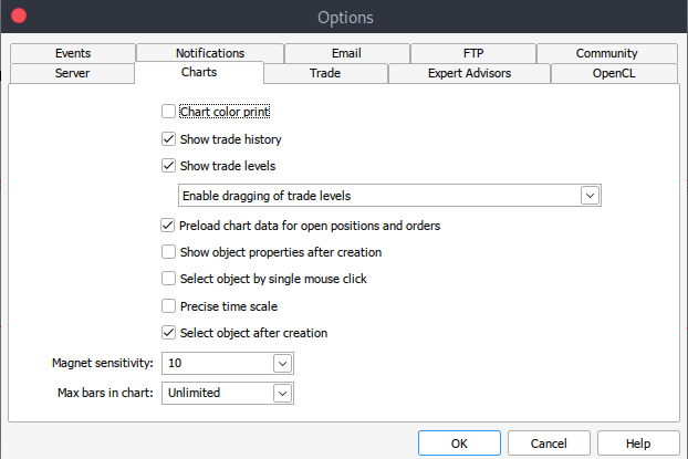
And if for some reason, you can't get historical data, you can retrieve it manually on your MetTrader5 platform with the following steps. Launch your MetaTrader platform and at the top of your MetaTrader 5 pane/panel navigate to > Tools and then > Options and you will land to the Charts options. You will then have to select the number of Bars in the chart you want to download. It's best to choose the option of unlimited bars since we'll be working with date, and we wouldn't know how many bars are there in a given period of time.

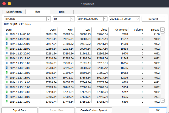
After that, you will now have to download the actual data. To do that, you will have to navigate to > View and then to  > Symbols, and you will land on the Specifications tab. Simply navigate to > Bars or Ticks depending on what kind of data want to download. Proceed and enter the start and end date period of the historical data you would like to download, after that, click on the request button to download the data and save it in the .csv format.

MetaTrader 5 Big Data Handling on Jupyter Lab

import pandas as pd

# Load the uploaded BTC 1H CSV file
file_path = '/home/int_junkie/Documents/DataVisuals/BTCUSD_H1.csv'
btc_data = pd.read_csv(file_path)

# Display basic information about the dataset
btc_data_info = btc_data.info()
btc_data_head = btc_data.head()

btc_data_info, btc_data_head

Output:

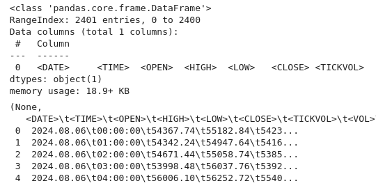
From the code above, as always, we inspect the data and understand the data set structure. We check the data types, shape, and completeness (using info()). We also get the dataset's content and layout (using head()). This is a common first step in exploratory data analysis to ensure the data is loaded correctly and to familiarize yourself with its structure.

# Reload the data with tab-separated values
btc_data = pd.read_csv(file_path, delimiter='\t')

# Display basic information and the first few rows after parsing
btc_data_info = btc_data.info()
btc_data_head = btc_data.head()

btc_data_info, btc_data_head

Output:

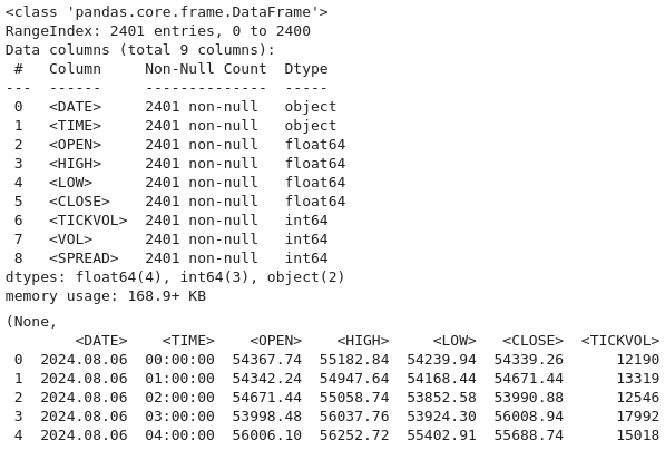
Now we use this code to reload the dataset from a file assumed to use tab-separated values (TSV) instead of the default comma-separated format. By specifying `delimiter=`\t`` in `pd.read-csv()` the data is correctly parsed into Pandas `DataFrame` for further analysis. We then use `btc-data-infor` to display metadata about the dataset, such as the number of rows, columns, data types, and any missing values.

# Combine <DATE> and <TIME> into a single datetime column and set it as the index
btc_data['DATETIME'] = pd.to_datetime(btc_data['<DATE>'] + ' ' + btc_data['<TIME>'])
btc_data.set_index('DATETIME', inplace=True)

# Drop the original <DATE> and <TIME> columns as they're no longer needed
btc_data.drop(columns=['<DATE>', '<TIME>'], inplace=True)

# Display the first few rows after modifications
btc_data.head()

Output:

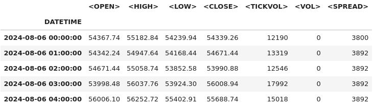
# Check for missing values and duplicates
missing_values = btc_data.isnull().sum()
duplicate_rows = btc_data.duplicated().sum()

# Clean data (if needed)
btc_data_cleaned = btc_data.drop_duplicates()

# Results
missing_values, duplicate_rows, btc_data_cleaned.shape

Output:

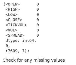
We can see from the output that we don't have any missing values from our dataset.

# Check for missing values
print("Missing values per column:\n", btc_data.isnull().sum())

# Check for duplicate rows
print("Number of duplicate rows:", btc_data.duplicated().sum())

# Drop duplicate rows if any
btc_data = btc_data.drop_duplicates()

Output:

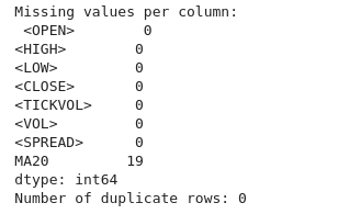
From the output, we can also see that we don't have any duplicated rows and columns.

# Calculate a 20-period moving average
btc_data['MA20'] = btc_data['<CLOSE>'].rolling(window=20).mean()
import ta

# Add RSI using the `ta` library
btc_data['RSI'] = ta.momentum.RSIIndicator(btc_data['<CLOSE>'], window=14).rsi()

Here, we compute a 20-period moving average and a 14-period RSI based on the closing prices from the `btc-data` Dataframe. These indicators, widely used in technical analysis, are added as new columns (MA-20 and RSI) for further analysis or visualization. These steps help traders identify trends and potential overbought or oversold conditions in the market.

import matplotlib.pyplot as plt

# Plot closing price and MA20
plt.figure(figsize=(12, 6))
plt.plot(btc_data.index, btc_data['<CLOSE>'], label='Close Price')
plt.plot(btc_data.index, btc_data['MA20'], label='20-period MA', color='orange')
plt.legend()
plt.title('BTC Closing Price and Moving Average')
plt.show()

Output:

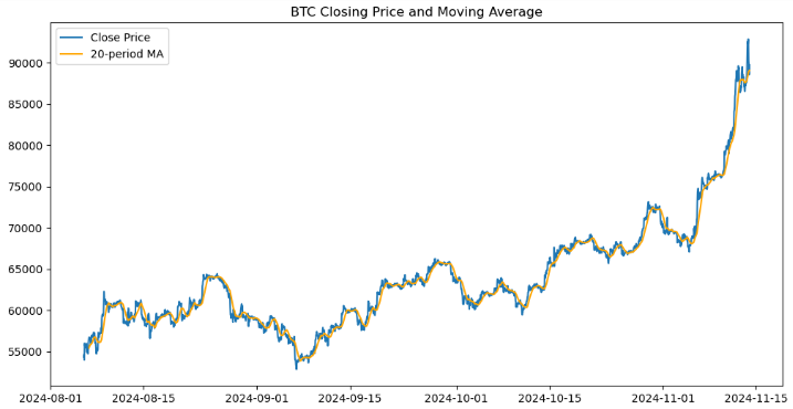
We created a visual representation of Bitcoin's closing prices and its 20-period moving average (MA20) using the Matplotlib library. It initializes a figure with a size of 12x6 inches and plots the closing prices against the DataFrame's index, labeling it as "Close Price." It overlays a second plot for the 20-period moving average in orange, labeled as "20-period MA." A legend is added to distinguish between the two lines, and the chart is titled "BTC Closing Price and Moving Average." Finally, the plot is displayed, offering a clear visualization of price trends and how they relate to the moving average.

import numpy as np
# Add log returns
btc_data['Log_Returns'] = (btc_data['<CLOSE>'] / btc_data['<CLOSE>'].shift(1)).apply(lambda x: np.log(x))

# Save the cleaned data
btc_data.to_csv('BTCUSD_H1_cleaned.csv')

Now we calculate the logarithmic returns of Bitcoin's closing prices and saves the updated dataset to a new CSV file. Logarithmic returns are computed by dividing each closing price by the previous period's closing price and applying the natural logarithm to the result. This is achieved using the `shift(1)`method to align each price with its predecessor, followed by applying a lambda function with `np.log`. The calculated values, stored in a new column named `Log-returns` provide a more analytically friendly measure of price changes, particularly useful in financial modeling and risk analysis. Finally, the updated dataset, including the newly added `Log-returns` column, we save it to a file named `BTCUSD-H1-cleaned.csv`, for further analysis.

import seaborn as sns
import matplotlib.pyplot as plt

# Correlation heatmap
sns.heatmap(btc_data.corr(), annot=True, cmap='coolwarm')
plt.title('Correlation Heatmap')
plt.show()

Output:

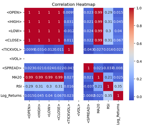
From the heat-map, we visualize the correlations between numerical columns in the `btc-data` Data frame using Seaborn and Matplotlib. The `btc-data.corr()` function computes pairwise correlation coefficients for all numerical columns, quantifying the linear relationships between them. The `sns.heatmap()` function displays this correlation matrix as a heatmap, with `annot=True` to display correlation values in each cell and `cmap='coolwarm'` to use a diverging color palette for easier interpretation. Warmer tones (red) represent positive correlations, while cooler tones (blue) indicate negative correlations. A title, "Correlation Heatmap," is added using Matplotlib, and the plot is displayed with `plt.show()`. This visualization helps identify patterns and relationships within the dataset at a glance.

from sklearn.model_selection import train_test_split

# Define features and target variable
X = btc_data.drop(columns=['<CLOSE>'])
y = btc_data['<CLOSE>']

# Split data
X_train, X_test, y_train, y_test = train_test_split(X, y, test_size=0.2, random_state=42)

We prepare the `btc-data` Data frame for machine learning by splitting it into training and testing subsets. First, the features `(x)` are defined by removing `<CLOSE>` column from the dataset, while the target variable `(y)` is set to the `<CLOSE>` column, representing the value to be predicted. The `train-test-split` function from Scikit-learn is then used to divide the data into training and testing sets, with 80% of the data allocated for training and 20% for testing, as specified by `test-size=0.2`. The `random-state=42` ensures the split is reproducible, maintaining consistency across different runs.

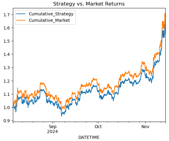
# Simple Moving Average Crossover Strategy
btc_data['Signal'] = (btc_data['MA20'] > btc_data['RSI']).astype(int)
btc_data['Returns'] = btc_data['<CLOSE>'].pct_change()
btc_data['Strategy_Returns'] = btc_data['Signal'].shift(1) * btc_data['Returns']

# Plot cumulative returns
btc_data['Cumulative_Strategy'] = (1 + btc_data['Strategy_Returns']).cumprod()
btc_data['Cumulative_Market'] = (1 + btc_data['Returns']).cumprod()

btc_data[['Cumulative_Strategy', 'Cumulative_Market']].plot(title='Strategy vs. Market Returns')
plt.show()

Output:

# Calculate short-term and long-term moving averages
btc_data['MA20'] = btc_data['<CLOSE>'].rolling(window=20).mean()
btc_data['MA50'] = btc_data['<CLOSE>'].rolling(window=50).mean()

# Generate signals: 1 for Buy, -1 for Sell
btc_data['Signal'] = 0
btc_data.loc[btc_data['MA20'] > btc_data['MA50'], 'Signal'] = 1
btc_data.loc[btc_data['MA20'] < btc_data['MA50'], 'Signal'] = -1

# Shift signal to avoid look-ahead bias
btc_data['Signal'] = btc_data['Signal'].shift(1)

# Calculate returns
btc_data['Returns'] = btc_data['<CLOSE>'].pct_change()
btc_data['Strategy_Returns'] = btc_data['Signal'] * btc_data['Returns']

# Calculate cumulative returns
btc_data['Cumulative_Market'] = (1 + btc_data['Returns']).cumprod()
btc_data['Cumulative_Strategy'] = (1 + btc_data['Strategy_Returns']).cumprod()

# Plot performance
import matplotlib.pyplot as plt

plt.figure(figsize=(12, 6))
plt.plot(btc_data['Cumulative_Market'], label='Market Returns')
plt.plot(btc_data['Cumulative_Strategy'], label='Strategy Returns')
plt.title('Strategy vs. Market Performance')
plt.legend()
plt.show()

Output:

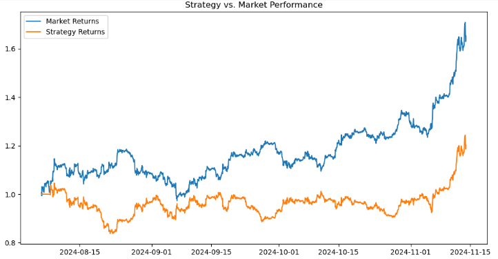
When evaluating the performance of a trading strategy compared to the market and visualize the results. First, we calculate the market returns as the percentage change in the `<CLOSE>` prices using `pct-change()` and store it in the `Returns` column. The strategy returns are computed by multiplying the `signal` column (representing trading signals such as 1 for buy, -1 for sell, or 0 for hold) with the market returns, storing the result in `strategy-returns`. Cumulative returns for both the market and the strategy are calculated using `(1 + returns).comprod()`, which simulates the compounded growth of $1 invested in the market `(Cumulative-market)` or following the strategy `(Cumulative-strategy)`.

# Add RSI
from ta.momentum import RSIIndicator

btc_data['RSI'] = RSIIndicator(btc_data['<CLOSE>'], window=14).rsi()

# Add MACD
from ta.trend import MACD

macd = MACD(btc_data['<CLOSE>'])
btc_data['MACD'] = macd.macd()
btc_data['MACD_Signal'] = macd.macd_signal()

# Target variable: 1 if next period's close > current close
btc_data['Target'] = (btc_data['<CLOSE>'].shift(-1) > btc_data['<CLOSE>']).astype(int)

from sklearn.model_selection import train_test_split
from sklearn.ensemble import RandomForestClassifier
from sklearn.metrics import accuracy_score, classification_report

# Define features and target
features = ['MA20', 'MA50', 'RSI', 'MACD', 'MACD_Signal']
X = btc_data.dropna()[features]
y = btc_data.dropna()['Target']

# Split data
X_train, X_test, y_train, y_test = train_test_split(X, y, test_size=0.2, random_state=42)

# Train a Random Forest Classifier
model = RandomForestClassifier(n_estimators=100, random_state=42)
model.fit(X_train, y_train)

# Evaluate the model
y_pred = model.predict(X_test)
print("Accuracy:", accuracy_score(y_test, y_pred))
print(classification_report(y_test, y_pred))

Output:

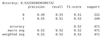
From the code above, we implement a machine learning pipeline to classify trading signals based on technical indicators using a Random Forest classifier. First, the feature set `(x)` is defined, including indicators such as the 20-period and 50-period moving averages `(MA20, MA50)`, Relative Strength Index (RSI), and MACD-related features `(MACD, MACD-Signals)`. The target variable `(y)` is set to the target `column`, which typically indicates buy, sell, or hold signals. Both `(x)` and `(y)` data is then split into training and testing sets, with 80% used for training and 20% for testing, ensuring consistency via `(random-state=42)`.

A Random Forest Classifier is initialized with 100 decision trees `(n-estimators=100)` and trained on the training data `(X-train and Y- train)`. The model’s predictions on the test set `(X-test)` are evaluated using accuracy score to determine its correctness and classification report to provide detailed metrics such as precision, recall, and F1-score for each class.

We then deploy the model using the following code:

import joblib

# Save the model
joblib.dump(model, 'btc_trading_model.pkl')

Putting it all together on MQL5

We are going to connect MQL5 to the python script that will be running our trained model, we will have to set up a communication channel between MQL5 and Python. In this case, we're going to use WebRequest.

//+------------------------------------------------------------------+
//|                                                BTC-Big-DataH.mq5 |
//|                                  Copyright 2024, MetaQuotes Ltd. |
//|                                             https://www.mql5.com |
//+------------------------------------------------------------------+
#property copyright "Copyright 2024, MetaQuotes Ltd."
#property link      "https://www.mql5.com"
#property version   "1.00"
#include <Trade\Trade.mqh>
CTrade trade;

All the necessary includes and the trading library (`trade.mqh`) for trade management.

// Function to get predictions from Python API
double GetPrediction(double &features[]) {
   // Convert the features array to a JSON-like string
   string jsonRequest = "[";
   for (int i = 0; i < ArraySize(features); i++) {
       jsonRequest += DoubleToString(features[i], 6);
       if (i != ArraySize(features) - 1) jsonRequest += ",";
   }
   jsonRequest += "]";
   
   // Define the WebRequest parameters
   string url = "http://127.0.0.1:5000/predict";
   string hdrs = {"Content-Type: application/json"}; // Add headers if needed
   char data[];
   StringToCharArray(jsonRequest, data); // Convert JSON request string to char array
   char response[];
   ulong result_headers_size = 0;


   //--------------------------------------------------------------------------------------
   string cookie=NULL;
   char post[], resultsss[];
   

   // Send the WebRequest
   int result = WebRequest("POST", url, cookie, NULL, 500, post, 0, resultsss, hdrs);
                          

   // Handle the response
   if (result == -1) {
       Print("Error sending WebRequest: ", GetLastError());
       return -1; // Return an error signal
   }

   // Convert response char array back to a string
   string responseString;
   CharArrayToString(response, (int)responseString);

   // Parse the response (assuming the server returns a numeric value)
   double prediction = StringToDouble(responseString);
   return prediction;
}

The function `GetPrediction()` sends a set of input features to a Python-based API and retrieve a prediction. The features are passed as an array of doubles, which are converted into a JSON-formatted string to match the API's expected input format. This conversion involves iterating through the feature array and appending each value to a JSON-like array structure. The `DoubleToString` function ensures the values are represented with six decimal places. The generated JSON string is then converted into a `char` array.

The function then prepares to make a POST request to the API endpoint `(http://127.0.0.1:5000/predict)` using web request. The required parameters are defined. Once the API response is received, it is converted back into a string using `CharArrayToString`. If the web request fails, an error is logged, and the function returns -1.

//+------------------------------------------------------------------+
//| Expert tick function                                             |
//+------------------------------------------------------------------+
void OnTick(){

   // Calculate indicators
   double MA20 = iMA(_Symbol, PERIOD_CURRENT, 20, 0, MODE_SMA, PRICE_CLOSE);
   double MA50 = iMA(_Symbol, PERIOD_CURRENT, 50, 0, MODE_SMA, PRICE_CLOSE);
   double RSI = iRSI(_Symbol, PERIOD_CURRENT, 14, PRICE_CLOSE);


   // Declare arrays to hold MACD data
   double MACD_Buffer[1], SignalLine_Buffer[1], Hist_Buffer[1];

   // Get MACD handle
   int macd_handle = iMACD(NULL, 0, 12, 26, 9, PRICE_CLOSE);
   if (macd_handle != INVALID_HANDLE) {
      // Copy the most recent MACD values into buffers
      if (CopyBuffer(macd_handle, 0, 0, 1, MACD_Buffer) <= 0) Print("Failed to copy MACD");
      if (CopyBuffer(macd_handle, 1, 0, 1, SignalLine_Buffer) <= 0) Print("Failed to copy Signal Line");
      if (CopyBuffer(macd_handle, 2, 0, 1, Hist_Buffer) <= 0) Print("Failed to copy Histogram");
   }
   
   // Assign the values from the buffers
   double MACD = MACD_Buffer[0];
   double SignalLine = SignalLine_Buffer[0];

   // Assign features
   double features[5];
   features[0] = MA20;
   features[1] = MA50;
   features[2] = RSI;
   features[3] = MACD;
   features[4] = SignalLine;

   // Get prediction
   double signal = GetPrediction(features);
   if (signal == 1){ 
      MBuy();  // Adjust lot size
   }
   else if (signal == -1){ 
      MSell();
   }
}

The `OnTick` begins by calculating key technical indicators: the 20-period and 50-period Simple Moving Averages (MA20 and MA50) to track trend direction, and the 14-period Relative Strength Index (RSI) to gauge market momentum. Additionally, it retrieves values for the MACD line, Signal line, and Histogram using the `iMACD` function, storing these values in buffers after validating the MACD handle. These computed indicators are assembled into a `features` array, which serves as input for a machine learning model accessed through the `GetPrediction` function. This model predicts a trading action, returning 1 for a buy signal or -1 for a sell signal. Based on the prediction, the function executes either a buy trade with `MBuy` or a sell trade with `MSell()`.

Python API

Below is a web API using Flask to serve predictions from a pre-trained machine learning model for BTC trading decisions.

from flask import Flask, request, jsonify
import joblib
import pandas as pd

# Load the model
model = joblib.load('btc_trading_model.pkl')

app = Flask(__name__)

@app.route('/predict', methods=['POST'])
def predict():
    data = request.json
    df = pd.DataFrame(data)
    prediction = model.predict(df)
    return jsonify(prediction.tolist())

app.run(port=5000)

Conclusion

In summary, we developed a comprehensive trading solution by combining big data handling, machine learning, and automation. Starting with historical BTC/USD data, we processed and cleaned it to extract meaningful features such as moving averages, RSI, and MACD. We used this processed data to train a machine learning model capable of predicting trading signals. The trained model was deployed as a Flask-based API, allowing external systems to query predictions. In MQL5, we implemented an Expert Advisor that collects real-time indicator values, sends them to the Flask API for predictions, and executes trades based on the returned signals.

This integrated trading solution empowers traders by combining the precision of technical indicators with the intelligence of machine learning. By leveraging a machine learning model trained on historical data, the system adapts to market dynamics, making informed predictions that can improve trading outcomes. The deployment of the model via an API enables flexibility, allowing traders to integrate it into diverse platforms like MQL5.