Statistical Arbitrage Through Cointegrated Stocks (Part 2): Expert Advisor, Backtests, and Optimization

Introduction

We have accepted the challenge of developing a framework for statistical arbitrage trading that can be used by the average retail trader. The core idea is to gather a set of statistical functions and methods of analysis to allow a retail trader with only a consumer notebook and a regular brokerage account to get started with statistical arbitrage for Forex, stocks, ETFs, and commodities.

We started with a simple correlation-based pairs trading that showed great potential on the backtest, but failed miserably on the demo account. It was not difficult to conclude that we were losing our trades at the order execution level. That is, our strategy was highly dependent on the order execution speed, but our infrastructure (consumer notebook, slow internet connection, and prototype code) was not even close to the required quality for this kind of arbitrage. Our entry/exit rules were highly dependent on timing, and our arbitrage opportunity was being closed even before our orders arrived at the broker server. 

We could try to solve, minimize, or circumvent the execution timing problem by setting a VPN (which we will be doing at some point in the future), by setting a professional account with maximum allowed slippage, or by trying to improve our prototype code. Each of these obvious and relatively cheap measures would have been of some help, and both together would certainly put our strategy back on track. But because we want to preserve our initial constraint of being useful to the average retail trader with minimum resources, instead of dealing with the execution speed, we set the goal of developing a strategy that would not be so dependent on execution speed. The implementation described below is one possible answer to this goal.

In the previous article, we introduced the Engle-Granger and the Johansen cointegration tests, their rationale from a trader's perspective, and their basic interpretation. Now we’ll be using them to build our cointegrated portfolio. 

Building a portfolio of cointegrated stocks

The drunk, the dog, and the random walk*

When researching cointegration, it is very common to stumble upon an analogy that explains pretty well the fundamental characteristic of cointegrated time series, or cointegrated stock prices, in this case. The analogy says that two non-cointegrated time series are like a drunk man walking with his dog. Their paths fall apart randomly, with no intrinsic, perceived, or measurable logic. The man and the dog can even arrive at home by different pathways, or the dog can even get lost forever.

But two cointegrated time series would be like if the dog were being conducted by a collar, that is, the man is still drunk, his steps are still dangling, but their paths go on together, no matter what. Cointegrated stocks are as if their prices were tied by an “invisible” collar. In the long run, they tend to arrive at home together. The home is the common mean, the mean spread.

But how can we find these cointegrated stocks in a universe of thousands of securities? Fortunately, we already know that some stocks from the same sector or industry tend to move together. This knowledge narrows down the initial to a more manageable number, but still a lot. 

Fig.1.  Number of symbols available on the MetaQuotes Demo server

Fig.2. Number of stock symbols available by country on a commercial broker demo server

There are several classic and “novel” methods already reviewed in the academic literature to filter the stock candidates for pair trading, but at the end of the day, none of them obtained better results than cointegration [Brunetti & De Luca, 2023].

Since our goal here is not an academic review but to backtest and describe a sample implementation, I adopted a simple heuristic to build our small portfolio.

“A heuristic (...) is any approach to problem solving that employs a pragmatic method that is not fully optimized, perfected, or rationalized, but is nevertheless 'good enough' as an approximation” (Wikipedia)

1. Cherry-pick some high liquidity Nasdaq stocks, all from semiconductor companies. You can start with a few dozen.
2. Among them, choose those most correlated to Nvidia on the daily timeframe for the last six months or less. Avoid longer lookback periods because we are interested in recent movements, and we are dealing with a very dynamic market (AI and semiconductors). Moreover, we will be updating our model on a monthly or weekly basis, so six months or less for this initial filter may put you on the right path.
3. Test the small group - the most correlated to Nvidia - for cointegration.
4. Once you find at least one significant Johansen vector, test the cointegrated spread for stationarity.
5. When you have a small group with at least one significant Johansen vector with a stationary cointegrated spread, get the first Johansen eigenvector to have the relative portfolio weights. 
6. Having the portfolio weights, you can backtest the cointegrated stock basket.

By using the Pearson correlation method we saw in the previous article, we narrowed down our basket to these three stocks listed below. All three companies have exposure to AI hardware demand and are part of the Nvidia supply chain directly or via adjacent markets.

Microchip Technology, Inc. (MCHP) - MCHP is not directly tied to Nvidia GPUs, but it benefits from the general semiconductor sector when there is rising demand for AI-related infrastructure like robotics and industrial AI via OEMs and system integrators for Nvidia-based systems.

Monolithic Power System Inc (MPWR) - MPWR supplies power management integrated circuits (PMICs) for servers and data centers. These PMICs are also used in high-performance Nvidia GPUs that require highly specialized power regulation to maintain thermal and electrical stability at high workloads. MPWR benefits from Nvidia's expansion into data centers and inference.

Micron Technology Inc. (MU) - MU supplies memory products, including High-Bandwidth Memory (HBM), which is crucial for AI accelerators like Nvidia’s H100. Its memory products are integrated in Nvidia GPUs and also in data center solutions. As Nvidia sells more AI chips, demand for Micron’s advanced memory soars. Micron announced strong AI-driven guidance in 2024–2025, tying its growth outlook directly to Nvidia’s performance.

The stocks we chose are not the most relevant information here. Instead, keep your focus on choosing the most correlated to the symbol you are taking as reference, that is, the basis of your hypothesis. In our case, it was NVDA, but it can be any symbol that fits your hypothesis.

We DO NOT want stocks that have an exceptionally high correlation with NVDA and low correlation among them. Instead, we want stocks that are highly correlated to NVDA and have a reasonably high correlation among themselves, too. In a sense, we want a correlated group of stocks around our reference because this property fits our hypothesis when we start cherry-picking: we are looking for a correlated basket.

We are looking for a Pearson Correlation Matrix like that.

	NVDA	MCHP	MPWR	MU
NVDA	1.000000	0.916887	0.894362	0.897219
MCHP	0.916887	1.000000	0.877042	0.941977
MPWR	0.894362	0.877042	1.000000	0.852675
MU	0.897219	0.941977	0.852675	1.000000

Table 1. Pearson Correlation Matrix between NVDA, MCHP, MPWR, and MU

This data can be more easily viewed as a seaborn heatmap.

import seaborn as sns
sns.heatmap(corr_matrix, annot=True, cmap="coolwarm")

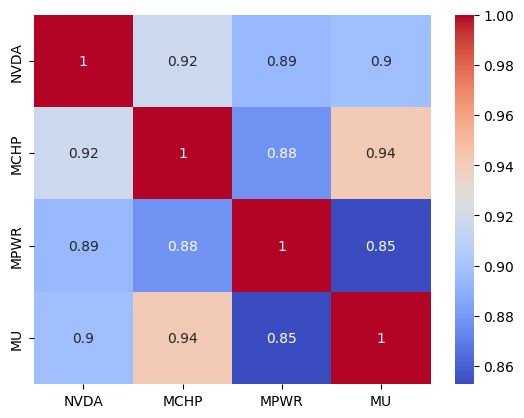
Fig.3. Pearson correlation matrix for NVDA, MCHP, MPWR, and MU viewed as a Seaborn heatmap

Note that although there is no exceptionally high correlation between MCHP, MPWR, and MU with NVDA, they are all moderately correlated with each other.

Note that while trading, we will need ticks from four assets to run the spread calculation that defines our entry and exit points. This is the main reason why we started cherry-picking high liquidity assets in the first place. We do not want illiquid assets that may go “out of sync” or drift from our OnTick event handler for more than a couple of seconds (see below).

Once we have this correlated basket defined, we run the Engle-Granger cointegration test to have an assessment of the cointegration level of the pairs and also the Johansen cointegration test to check the cointegration level of the basket, that is, the cointegration level of the group of assets. You can refer to the previous article for a more detailed description of these two tests.

Then we get the portfolio hedge ratios from the Johansen eigenvector.

🧮 Portfolio Weights (Johansen Eigenvector):

MU 2.699439

NVDA1.000000

MPWR-1.877447

MCHP-2.505294

The Johansen Eigenvector is a list of numbers, one for each stock in your group, that tells you the weight or importance of each stock in maintaining the stable relationship identified by the Johansen test. These weights ensure that when you combine the stocks, by buying or selling them in specific proportions, their combined price movements form a somewhat predictable, more or less stable pattern.

These values will be used to balance our order volume and minimize our market exposure. Remember that in statistical arbitrage strategies, we are always looking for market neutrality. We can think of a weighted portfolio as an improvement over that simple pairs trading technique, where we buy/sell one unit of each symbol at the same time.

You will find these portfolio weights among the global variables of our sample Expert Advisor.

// Global variables
string symbols[] = {"MU", "NVDA", "MPWR", "MCHP"}; // Asset symbols
double weights[] = {2.699439, 1.000000, -1.877447, -2.505294}; // Johansen eigenvector

NVDA has the value 1.0 because we chose to normalize on the symbols list first asset in our Python code (attached), which is NVDA. Normalization allows us to have a relative interpretation of the other values. You can choose to normalize on any other symbol on the Python list. It is an arbitrary reference.

# === FIRST COINTEGRATION VECTOR ===
v = johansen_result.evec[:, 0]
# v = v / v[-1]  # Normalize on symbols list last asset
v = v / v[0] # Normalize on symbols list first asset

Now we can test the multivariate spread for stationarity.

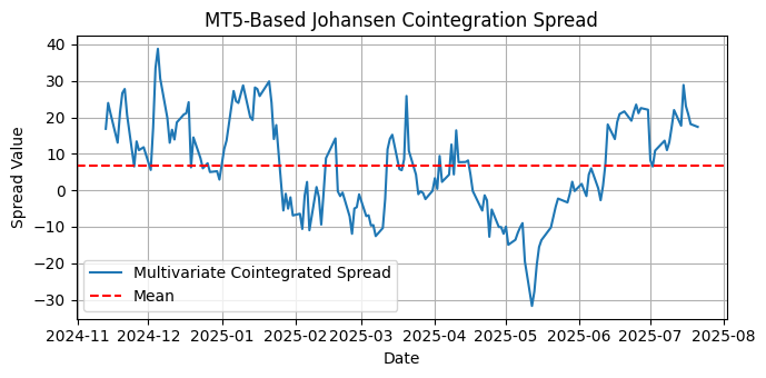
Fig.4. Plot of multivariate cointegrated spread for NVDA, MCHP, MPWR, and MU

The visual inspection of the multivariate spread is a valid way to assess its suitability to be used in a mean-reversion strategy. The visual inspection allows us to have a quick estimation of the spread distribution around the mean, the spread return to the mean, and its possible stationarity. The absence of a visual trend is a strong clue for stationarity, as is the absence of seasonality.

But the visual inspection is not enough and cannot be used in automated models and portfolio updates. Fortunately, we have the Augmented Dickey Fuller (“ADF”) and the Kwiatkowski-Phillips-Schmidt-Shin (“KPSS”) tests to come to our rescue.

Use the ADF and KPSS tests to confirm that the spread is mean-reverting.

# Augmented Dickey-Fuller Test
from statsmodels.tsa.stattools import adfuller

adf_result = adfuller(spread, regression='c')  # 'ct' for trend and constant
print("ADF Test on Spread:")
print(f"  ADF Statistic : {adf_result[0]:.4f}")
print(f"  p-value       : {adf_result[1]:.4f}")
print(f"  Critical Values:")
for key, value in adf_result[4].items():
    print(f"    {key}: {value:.4f}")

if adf_result[1] < 0.05:
    print("\n✅ The cointegrated spread is stationary (reject the null hypothesis).")
else:
    print("\n❌ The cointegrated spread is NOT stationary (fail to reject the null hypothesis).")

ADF Test on Spread:

  ADF Statistic: -3.2331  

  p-value: 0.0181

  Critical Values:

    1%: -3.4704    

    5%: -2.8791

    10%: -2.5761

✅ The cointegrated spread is stationary (reject the null hypothesis).

# KPSS Test
from statsmodels.tsa.stattools import kpss

def run_kpss(series, regression='c'):
    statistic, p_value, lags, crit_values = kpss(series, regression=regression, nlags='auto')
    print("KPSS Test on Spread:")

KPSS Test on Spread:

  KPSS Statistic: 0.4142  

  p-value: 0.0710  

  Lags Used: 8

  Critical Values:

    10%: 0.347    

    5%: 0.463    

    2.5%: 0.574

    1%: 0.739

✅ The cointegrated spread is stationary (fail to reject null of stationarity).

This step is critical. Without a stationary spread, our mean-reverting hypothesis falls to pieces. Without a stationary spread, prices may keep going apart, and we may be left with dangling positions that never close properly by mean reversion. Asserting that the spread is stationary is critical in this kind of strategy.

Later, as our statistical arbitrage framework evolves, we will be rotating our portfolio in automated ways. Thus, having these stationarity tests in our toolkit is paramount because we cannot rely only on the visual assessment of plots. 

The sample implementation

Our sample implementation starts by defining thresholds for entry/exit points in the form of standard deviations from the mean.

// Input parameters
input double EntryThreshold = 2.0;      // Entry threshold (standard deviations)
input double ExitThreshold = 0.3;       // Exit threshold (standard deviations)
input double LotSize = 10.0;            // Fixed lot size per leg
input int LookbackPeriod = 252;         // Lookback for moving average/standard deviation
input int Slippage = 3;                 // Max allowed slippage

The 10.0 units default lot size should make it easy to check the portfolio weights in the orders while backtesting.

The max allowed slippage is almost decorative here, because we are developing for the average retail trader, and max allowed slippage is, usually, a feature only available to professional trading accounts. But it does no harm to have it in place for future improvements. The parameter will simply be ignored by the broker server if the trading account has this feature disabled.

The lookback period used for the calculation of the moving average and the standard deviations may be the same period used for the correlation and cointegration tests, but this is not a requirement. Once we have spotted a cointegration on the daily timeframe for the last six months, there is no problem in operating on the hourly timeframe for a two-week lookback period, for example. The system is flexible enough to allow for experimentation, and in this flexibility lies a plethora of opportunities.

Some notes about specific code functions.

OnInit()

// Check if all symbols are available
   for(int i = 0; i < ArraySize(symbols); i++)
     {
      if(!SymbolSelect(symbols[i], true))
        {
         Print("Error: Symbol ", symbols[i], " not found!");
         return(INIT_FAILED);
        }
     }

We check if all the symbols in our basket are available on Market Watch for the quotes request.

// Set a timer for spread, mean, and stdev calculations
   EventSetTimer(1); // one second

We set a timer for the spread, mean, and standard deviation calculations outside of the OnTick() function. That is because, as you probably know, the OnTick event handler is tied to the chart/symbol where the EA is launched. While there are no updates for this symbol, the OnTick is not triggered. We do not want to be dependent on these updates. By using a timer, in this case with a one-second interval, we can be sure that at this interval we will check for new quotes. We are moving from a passive quote updating to an active quote updating. 

OnTimer()

void OnTimer(void)
  {
// Calculate current spread value
   currentSpread = CalculateSpread();
// Update spread buffer (rolling window)
   static int barCount = 0;
   if(barCount < LookbackPeriod)
     {
      spreadBuffer[barCount] = currentSpread;
      barCount++;
      return; // Wait until buffer is filled
     }
// Shift buffer (remove oldest value, add newest)
   for(int i = 0; i < LookbackPeriod - 1; i++)
      spreadBuffer[i] = spreadBuffer[i + 1];
   spreadBuffer[LookbackPeriod - 1] = currentSpread;
// Calculate mean and standard deviation using custom functions
   spreadMean = CalculateMA(spreadBuffer, LookbackPeriod);
   spreadStdDev = CalculateStdDev(spreadBuffer, LookbackPeriod, spreadMean);
  }

In the OnTimer event handler, we iterate over the chart lookback period to calculate the spread, the mean, and the standard deviation.

OnTick()

void OnTick()
  {
// Trading logic
   if(!tradeOpen)
     {
      // Check for entry signal (spread deviates from mean)
      if(currentSpread > spreadMean + EntryThreshold * spreadStdDev)
        {
         // Short spread (sell MU/NVDA, buy MPWR/MCHP)
         ExecuteTrade(ORDER_TYPE_SELL);
         tradeOpen = true;
        }
      else
         if(currentSpread < spreadMean - EntryThreshold * spreadStdDev)
           {
            // Buy spread (buy MU/NVDA, sell MPWR/MCHP)
            ExecuteTrade(ORDER_TYPE_BUY);
            tradeOpen = true;
           }
     }
   else
     {
      // Check for exit signal (spread reverts to mean)
      if((currentSpread <= spreadMean + ExitThreshold * spreadStdDev) &&
         (currentSpread >= spreadMean - ExitThreshold * spreadStdDev))
        {
         CloseAllTrades();
         tradeOpen = false;
        }
     }
// Display spread in chart
   Comment(StringFormat("Spread: %.2f | Mean: %.2f | StdDev: %.2f", currentSpread, spreadMean, spreadStdDev));
  }

The OnTick() event handler has the trading logic only. If we are not in the market (!tradeOpen()), and we have a trading signal, we buy or sell according to the portfolio weights we received from the Johansen eigenvector.

ExecuteTrade(ENUM_ORDER_TYPE orderType)

//+------------------------------------------------------------------+
//| Execute trade with normalized integer lots                |
//+------------------------------------------------------------------+
void ExecuteTrade(ENUM_ORDER_TYPE orderType)
  {
   double volumeArray[];
   ArrayResize(volumeArray, ArraySize(symbols));
   if(!NormalizeVolumeToIntegerLots(volumeArray, symbols, weights, LotSize))
     {
      Print("Volume normalization failed!");
      return;
     }
   for(int i = 0; i < ArraySize(symbols); i++)
     {
      ENUM_ORDER_TYPE legType = (weights[i] > 0) ? orderType :
                                (orderType == ORDER_TYPE_BUY ? ORDER_TYPE_SELL : ORDER_TYPE_BUY);
      trade.PositionOpen(symbols[i], legType, volumeArray[i], 0, 0, 0, "NVDA Coint");
     }
  }

(...)

//+------------------------------------------------------------------+
//| Normalize volumes to integer lots                             |
//+------------------------------------------------------------------+
bool NormalizeVolumeToIntegerLots(double &volumeArray[], const string &symbols_arr[], const double &weights_arr[], double baseLotSize)
  {
   MqlTick tick; // Structure to store bid/ask prices
   double totalDollarExposure = 0.0;
   double dollarExposures[];
   ArrayResize(dollarExposures, ArraySize(symbols_arr));
// Step 1: Calculate dollar exposure for each leg
   for(int i = 0; i < ArraySize(symbols_arr); i++)
     {
      if(!SymbolInfoTick(symbols_arr[i], tick)) // Get latest bid/ask
        {
         Print("Failed to get price for ", symbols_arr[i]);
         return false;
        }
      // Use bid price for short legs, ask for long legs
      double price = (weights_arr[i] > 0) ? tick.ask : tick.bid;
      dollarExposures[i] = MathAbs(weights_arr[i]) * price * baseLotSize;
      totalDollarExposure += dollarExposures[i];
     }
// Step 2: Convert dollar exposure to integer lots
   for(int i = 0; i < ArraySize(symbols_arr); i++)
     {
      double ratio = dollarExposures[i] / totalDollarExposure;
      double targetDollarExposure = ratio * totalDollarExposure;
      // Get min/max lot size and step for the symbol
      double minLot = SymbolInfoDouble(symbols_arr[i], SYMBOL_VOLUME_MIN);
      double maxLot = SymbolInfoDouble(symbols_arr[i], SYMBOL_VOLUME_MAX);
      double lotStep = SymbolInfoDouble(symbols_arr[i], SYMBOL_VOLUME_STEP);
      // Get current price again (for lot calculation)
      if(!SymbolInfoTick(symbols_arr[i], tick))
         return false;
      double price = (weights_arr[i] > 0) ? tick.ask : tick.bid;
      double lots = targetDollarExposure / price;
      lots = MathFloor(lots / lotStep) * lotStep; // Round down to nearest step
      // Clamp to broker constraints using custom Clamp()
      volumeArray[i] = Clamp(lots, minLot, maxLot);
     }
   return true;
  }

The backtest

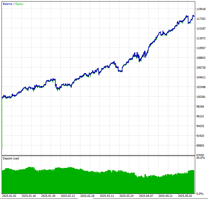
Fig.5. Equity curve from Nasdaq cointegrated basket backtest for the first five months of 2025 on the daily timeframe

The equity curve shows that our hypothesis is viable, although it requires a not-yet-implemented money management strategy to avoid some aggressive drawdowns.

Fig.6. Backtest summary from Nasdaq cointegrated basket for the first five months of 2025 on the daily timeframe

As you can see, our price history quality is very low, but it is what we have for free for these four stock symbols, so we are working with what we have. When implementing this strategy for real money trading, it is strongly recommended that you look for more quality in your price history.

Fig.7. Backtest entries by periods from the Nasdaq cointegrated basket backtest for the first five months of 2025 on the daily timeframe

Fig.8. Holding times from the Nasdaq cointegrated basket backtest for the first five months of 2025 on the daily timeframe

The average position holding of ~20 min seems to be good because we are avoiding those one-to-two-second position holdings from our first (and failed) attempt described in the first part of this article.

Fig.9. MFE and MAE from the Nasdaq cointegrated basket backtest for the first five months of 2025 on the daily timeframe

Cointegration beyond stocks

These are somewhat satisfactory results for our first same sector cointegrated stocks basket. With some improvements like proper money management and better quality data for optimizations, we can expect to have a reasonable candidate to test in a demo account for a couple of weeks.

But as you probably already realized, it is a very generic solution in which we are using only a very small subset of Nasdaq stocks in a yet smaller combination of cointegration test lookback period and timeframe. That is, we are using four symbols that were tested for cointegration in the last six months in the daily timeframe. If you start combining these parameters, you may find dozens of opportunities that may be worth some attention.

Besides that, you are not limited to Nasdaq stocks or even limited to stocks. You may try multi-asset cointegration tests between stocks and ETFs or sector indexes.

Some examples

Here are some examples of cointegration tested for the last six months (180 days) on the daily timeframe.

Gold-related ETFs

symbols = ['AAAU', 'USGO', 'BGLD']

1. AAAU – Goldman Sachs Physical Gold ETF

“AAAU is an exchange-traded fund that seeks to reflect the performance of the price of gold bullion. The fund holds physical gold bars stored in secure vaults, and investors can redeem shares for actual gold (subject to conditions). AAAU is designed to provide direct exposure to gold prices with minimal tracking error and no derivatives.”

2. USGO – Abrdn Physical Gold Shares ETF

“USGO is a physically backed gold ETF managed by Aberdeen Investments. Like AAAU, it aims to track the price of gold bullion by holding allocated physical gold stored in secure vaults. It offers investors a simple and cost-effective way to gain exposure to gold without taking physical delivery themselves.”

3. BGLD – FT Vest Gold Strategy Target Income ETF

“BGLD is an actively managed gold strategy ETF that seeks to provide income and exposure to gold. Unlike AAAU and USGO, BGLD does not directly hold physical gold. Instead, it uses a combination of gold-related derivatives (such as futures and options) and income-generating strategies to deliver targeted returns with gold-like behavior and a focus on generating monthly income.”

Index(['AAAU', 'USGO', 'BGLD'], dtype='object')

Engle-Granger Cointegration Test Results:

AAAU and USGO | p-value: 0.1322

AAAU and BGLD | p-value: 0.0209

USGO and BGLD | p-value: 0.0144

Most cointegrated pair (Engle-Granger): USGO and BGLD | p-value: 0.0144

Remember that the Engle-Granger tests only pairwise relationships. This test will not indicate whole basket interactions that the Johansen test captures.

Johansen Test Results (Trace Statistic):

Number of observations: 119

Number of variables: 3

Rank 0: Trace Stat = 30.21 | 5% CV = 29.80 | Significant

Rank 1: Trace Stat = 10.65 | 5% CV = 15.49 | Not significant

Rank 2: Trace Stat = 4.25 | 5% CV = 3.84 | Significant

With the Johansen test, we can see the number of cointegrating relationships in the whole basket at each rank.

At rank 0, the trace statistic (30.21) exceeds the 5% critical value (29.80), indicating that at least one cointegrating vector exists. At rank 1, the test is not significant, but at rank 2, it is again significant (4.25 > 3.84), implying a second cointegrating relationship.

In the Engle-Granger result, we can see that AAAU-BGLD (p = 0.0209) and USGO-BGLD (p = 0.0144) are both significantly ‘more cointegrated’ than AAAU-USGO (p = 0.1322), indicating that two independent cointegrating vectors exist among the three assets, and probably a strong and stable long-term equilibrium relationship in the basket.

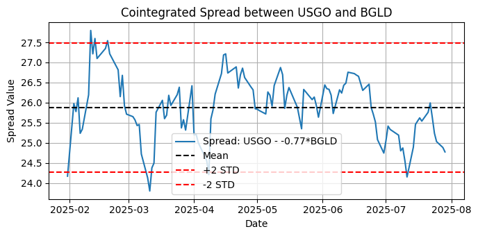
Fig.10. Plot of the cointegrated spread between USGO and BGLD for the last six months on the daily timeframe

ADF Test on Spread:

  ADF Statistic: -3.7659 

  p-value: 0.0033

  Critical Values:

    1%: -3.4870   

    5%: -2.8864

    10%: -2.5800

✅ The spread is stationary (reject the null hypothesis).

KPSS Test on Spread:

  KPSS Statistic: 0.1910 

  p-value: 0.1000  Lags Used: 5

  Critical Values:

    10%: 0.347   

    5%: 0.463   

    2.5%: 0.574

    1%: 0.739

✅ The spread is stationary (fail to reject null of stationarity).

We can see that BGLD has a strong cointegrating relationship with both AAAU and USGO and with the stationarity of the spread between USGO-BGLD confirmed, we know that we have a strong indication that these assets are good candidates for a gold-related cointegrated basket.

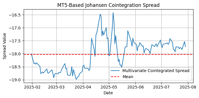
Fig.11. Plot of multivariate cointegrated spread between AAAU, USGO, and BGLD for the last six months on the daily timeframe

However, their cointegrated spread is not stationary for this period and timeframe. 

ADF Test on Spread:

  ADF Statistic: -2.7186 

  p-value: 0.0709

  Critical Values:

    1%: -3.4870   

    5%: -2.8864

    10%: -2.5800

❌ The cointegrated spread is NOT stationary (fail to reject the null hypothesis).

KPSS Test on Spread:

  KPSS Statistic: 0.9687 

  p-value: 0.0100  Lags Used: 6

  Critical Values:

    10%: 0.347   

    5%: 0.463   

    2.5%: 0.574

    1%: 0.739

❌ The cointegrated spread is NOT stationary (reject null of stationarity).

Silver-related ETFs

symbols = ['CEF', 'SLV', 'SIVR']

1. CEF – Sprott Physical Gold and Silver Trust

“A closed-end trust that holds both physical gold and silver bullion. It trades at a premium or discount to its net asset value and is not a pure silver play, making it structurally different from SLV and SIVR.”

2. SLV – iShares Silver Trust

“A physically backed silver ETF that seeks to reflect the performance of the price of silver bullion. It is one of the largest and most liquid silver ETFs.”

3. SIVR – Aberdeen Physical Silver Shares ETF

“Similar to SLV, SIVR is a physically backed silver ETF, but typically has a lower expense ratio, making it attractive for cost-sensitive investors.”

Index(['CEF', 'SLV', 'SIVR'], dtype='object')

Engle-Granger Cointegration Test Results:

CEF and SLV | p-value: 0.6092
CEF and SIVR | p-value: 0.6109

SLV and SIVR | p-value: 0.0000

Most cointegrated pair (Engle-Granger): SLV and SIVR | p-value: 0.0000

Johansen Test Results (Trace Statistic):

Number of observations: 121

Number of variables: 3

Rank 0: Trace Stat = 62.67 | 5% CV = 29.80 | Significant

Rank 1: Trace Stat = 7.20 | 5% CV = 15.49 | Not significant

Rank 2: Trace Stat = 1.95 | 5% CV = 3.84 | Not significant

At rank 0 (62.67 > 29.80), the trace statistic is significant, indicating the presence of at least one cointegrating vector among the three silver-related ETFs. However, the ranks 1 and 2 are not significant, indicating that there is only one stable long-term relationship shared by this basket.

The Engle-Granger results show that the pair SLV and SIVR has a strong cointegration signal (p = 0.0000). The CEF does not appear cointegrated with either SLV or SIVR (p > 0.6). Looking again at the Johansen result, we can infer that the cointegration likely comes from the close relationship between SLV and SIVR, since they are nearly perfect substitutes, both physically backed silver ETFs, which justifies their cointegration. CEF is silver-exposed but also provides exposure to gold and is a closed-end fund. Thus, it behaves differently.

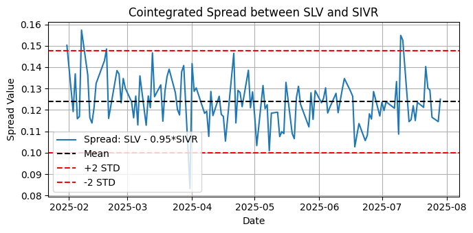
Fig.12. Plot of the cointegrated spread between SLV and SIVR for the last six months on the daily timeframe

ADF Test on Spread:

  ADF Statistic: -11.0833 

  p-value: 0.0000

  Critical Values:

    1%: -3.4861   

    5%: -2.8859

    10%: -2.5798

✅ The spread is stationary (reject the null hypothesis).

KPSS Test on Spread:

  KPSS Statistic: 0.6246 

  p-value: 0.0204  Lags Used: 1

  Critical Values:

    10%: 0.347   

    5%: 0.463   

    2.5%: 0.574

    1%: 0.739

❌ The spread is NOT stationary (reject null of stationarity).

Here we found that the cointegrated spread between SLV and SIVR is stationary per the ADF test but non-stationary per the KPSS.  We saw a similar example in the previous article, with the corresponding explanation from statsmodels library documentation about how to interpret these kinds of contradictory results.

“Case 1: Both tests conclude that the series is not stationary - The series is not stationary

Case 2: Both tests conclude that the series is stationary - The series is stationary

Case 3: KPSS indicates stationarity and ADF indicates non-stationarity - The series is trend stationary. The trend needs to be removed to make the series strict stationary. The detrended series is checked for stationarity.

Case 4: KPSS indicates non-stationarity and ADF indicates stationarity - The series is difference stationary. Differencing is to be used to make series stationary. The differenced series is checked for stationarity.”

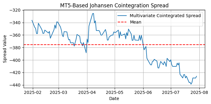
Fig.13. Plot of multivariate cointegrated spread between CEF, SLV, and SIVR for the last six months on the daily timeframe

For the multivariate cointegrated spread, that is, the whole basket, the plot shows that the spread is NOT mean-reverting for this period and timeframe. The stationarity test will confirm.

ADF Test on Spread:

  ADF Statistic: -0.8780 

  p-value: 0.7951

  Critical Values:

    1%: -3.4865   

    5%: -2.8862

    10%: -2.5799

❌ The cointegrated spread is NOT stationary (fail to reject the null hypothesis).

KPSS Test on Spread:

  KPSS Statistic: 1.3918 

  p-value: 0.0100 

  Lags Used: 6

  Critical Values:

    10%: 0.347   

    5%: 0.463   

    2.5%: 0.574

    1%: 0.739

❌ The cointegrated spread is NOT stationary (reject null of stationarity).

What does this mean? Certainly, we do not have a suitable basket of silver-related ETFs here, but we have two highly cointegrated ETFs (SLV and SIVR) that may be worth a close look for pairs trading, which is the subject of our premier article of this series.

These two examples aim to make it clear that when looking for cointegrated assets for statistical arbitrage opportunities, experimentation and research are the keywords. Also, we should keep in mind that statistics alone are not a replacement for your understanding of the sector and market knowledge.

Conclusion

This article describes a sample Expert Advisor being backtested over a small group of cointegrated stocks. It is the second of two articles describing the most common statistical measures for statistical arbitrage portfolio building: correlation coefficients and cointegration evaluation, along with spread stationarity testing.

It’s worth noting that this kind of strategy, although almost impossible to use for currencies (FX pairs) due to the rare condition of more than two cointegrated currencies being found, also applies to indices, ETFs, and commodities. 

Now that we have the basic tools for cointegration-based portfolio building, the logical next steps could be the implementation of a real-time portfolio rotation, eventually evolving to a machine learning approach in the future.

References

Marianna Brunetti & Roberta De Luca, 2023. "Pre-selection in cointegration-based pairs trading," Statistical Methods & Applications, Springer; Società Italiana di Statistica, vol. 32(5), pages 1611-1640, December.

Notes

* Although the analogy is probably derived from, the random walk here should not be confused with Pearson’s Random Walk, the stochastic process described and named by the English mathematician.

Attached file	Description
corr_pearson.ypng	This file is a Jupyter notebook containing Python code. The script runs the Pearson correlation test.
coint_stocks_ETFs.ypnb	This file is also a Jupyter notebook containing Python code. The script runs the Engle-Granger, the Johansen cointegration tests, and the ADF and KPSS stationarity tests.
Nasdaq_NVDA_Coint.mql5	This file contains the sample Expert Advisor used in the backtests.
Nasdaq_NVDA_Coint.ini	This file is a configuration settings file (.ini) containing the parameter used in the backtest.
Nasdaq_NVDA_Coint.NVDA.Daily.20250101_20250515.021.ini	This file is also a configuration settings file (.ini) containing the optimization parameters used in the backtest.