Build Self Optimizing Expert Advisors in MQL5 (Part 4): Dynamic Position Sizing

Electronic and Digital Computers have been around since the 1950s, but financial markets have existed for centuries. Human traders have historically succeeded without advanced computational tools, presenting a challenge in designing modern trading software. Should we leverage full computational power or align with successful human trading principles? This article advocates for balancing simplicity with modern technology. Despite today's advanced tools, many traders have succeeded in complex decentralized systems without high-powered software like MQL5 API. 

Most of the day-to-day decision-making processes that we use as humans, can be challenging to meaningfully convey to a computer. For example, when trading, it is common to hear someone remark “I was very confident about my decision, so I increased the lot size”. How can we instruct our trading applications to do the same and increase the position size if it feels “confident” about the trade?

I hope it is immediately obvious to the reader that one cannot attain this goal, without introducing complexity into the system to measure how “confident” the computer “feels”. One approach is to build probabilistic models to quantify the “confidence” of a trade. In this article, we’ll build a simple logistic regression model to measure the confidence of our trades, allowing our application to independently scale our positions.

We will focus on the Bollinger Bands strategy, as originally proposed by John Bollinger. We aim to refine this strategy, addressing its shortcomings without losing the essence of the idea. 

Our trading application will aim to:

1. Place an additional trade with a larger lot size if the model is confident in the trade
2. Place a single trade with a smaller lot size if the model is less confident

The original trading strategy as proposed by John Bollinger placed 493 trades in our back-test of the strategy. Of all the trades placed, 62% were profitable. Although this is a healthy proportion of winning trades, it wasn't enough to produce a profitable trading strategy. We lost -$813 over our back-test period and produced a Sharpe ratio of -0.33. Our refined version of the algorithm placed 495 trades in total, with 63% of all trades being profitable. Our total profit at the end of the back-test increased dramatically to $2 427 over the same period of time and our Sharpe ratio settled at 0.74. 

The goal of this article is not to undermine the power of advanced computational tools, such as DNNs or reinforcement learning algorithms. On the contrary, I am deeply excited by the possibilities these technologies bring to the table. However, it’s important to recognize that complexity for its own sake does not necessarily lead to better outcomes.

I understand the challenges that come with being a new member of an algorithmic trading community. I’ve been there myself, full of ambition but unsure how to get started. It’s easy to feel overwhelmed by the vast number of tools, techniques and options that are available at your fingertips.
This article is meant to provide a roadmap for those who are just beginning. By starting simple, you can build the confidence to tackle more complex problems on your own, with a more profound understanding of their application. We obtained the results published in this article by preserving the original and simple trading rules suggested by John Bollinger and supplementing them with complexity to emulate the human decision-making process, as opposed to introducing complexity for its own sake.

Overview of The Trading Strategy

Fig 1: An image of our Bollinger Band Strategy in action

Our trading strategy is based on following the trading signals proposed by John Bollinger. The original rules of the strategy are satisfied if we sell whenever price levels breach the top Bollinger Band, and we will buy if price levels fall beneath the lower band.

Generally speaking, we can extend these rules to also serve as our exit conditions. As to say that whenever price levels appear above the uppermost band, we will close any buy trades that may be open in addition to opening our sell trades. These sets of rules are enough to create a self-managing system that knows when to open and close its positions on its own. 

We will test our trading strategy on the GBPUSD Pair from 1 January 2022 until 30 December 2024 on the M15 time frame. 

Getting Started in MQL5

To get the ball rolling in MQL5, we begin by first defining system constants, such as the intended pair to be traded, the lot size to be used and other constants that we do not want the user to change.

//+------------------------------------------------------------------+
//|                                 GBPUSD BB Breakout Benchmark.mq5 |
//|                                               Gamuchirai Ndawana |
//|                    https://www.mql5.com/en/users/gamuchiraindawa |
//+------------------------------------------------------------------+
#property copyright "Gamuchirai Ndawana"
#property link      "https://www.mql5.com/en/users/gamuchiraindawa"
#property version   "1.00"

//+------------------------------------------------------------------+
//| System constants                                                 |
//+------------------------------------------------------------------+
#define BB_SHIFT  0                         // Our bollinger band should not be shifted
#define SYMBOL    "GBPUSD"                  // The intended pair for our trading system
#define BB_PRICE  PRICE_CLOSE               // The price our bollinger band should work on
#define LOT       0.1                       // Our intended lot size

From there, let us load the trade library.

//+------------------------------------------------------------------+
//| Dependencies                                                     |
//+------------------------------------------------------------------+
#include <Trade\Trade.mqh>
CTrade Trade;

Some aspects of the trading strategy may be controlled by the end user, such as the time frame we should use for our technical indicator calculations and the period for the Bollinger Bands indicator.

//+------------------------------------------------------------------+
//| User inputs                                                      |
//+------------------------------------------------------------------+
input group "Technical Indicators"
input ENUM_TIMEFRAMES TF = PERIOD_M15;   // Intended time frame
input int    BB_PERIOD   = 30;               // The period for our bollinger bands
input double BB_SD       = 2.0;              // The standard deviation for our bollinger bands

We shall also need to define global variables used throughout our program.

//+------------------------------------------------------------------+
//| Global variables                                                 |
//+------------------------------------------------------------------+

//+------------------------------------------------------------------+
//| Technical indicators                                             |
//+------------------------------------------------------------------+
int    bb_handler;
double bb_u[],bb_m[],bb_l[];

//+------------------------------------------------------------------+
//| System variables                                                 |
//+------------------------------------------------------------------+
int state;
double o,h,l,c,bid,ask;

When our trading application is loaded for the first time, we shall call our initialization function.

//+------------------------------------------------------------------+
//| Expert initialization function                                   |
//+------------------------------------------------------------------+
int OnInit()
  {
//--- Setup our system
   if(!setup())
      return(INIT_FAILED);
//---
   return(INIT_SUCCEEDED);
  }

If our application is no longer in use, we shall release the technical indicators we aren't using.

//+------------------------------------------------------------------+
//| Expert deinitialization function                                 |
//+------------------------------------------------------------------+
void OnDeinit(const int reason)
  {
//--- Release resources we no longer need
   release();
  }

Upon receiving updated price information, we need to store the new price data and process it to make a trading decision.

//+------------------------------------------------------------------+
//| Expert tick function                                             |
//+------------------------------------------------------------------+
void OnTick()
  {
//--- Update our system variables
   update();
  }
//+------------------------------------------------------------------+

This function is responsible for setting up our technical indicator.

//+------------------------------------------------------------------+
//| Custom functions                                                 |
//+------------------------------------------------------------------+

//+------------------------------------------------------------------+
//| Setup our technical indicators and other variables               |
//+------------------------------------------------------------------+
bool setup(void)
  {
//--- Setup our system
   bb_handler = iBands(SYMBOL,TF,BB_PERIOD,BB_SHIFT,BB_SD,BB_PRICE);
   state = 0;

//--- Validate our system has been setup correctly
   if((bb_handler != INVALID_HANDLE) && (Symbol() == SYMBOL))
      return(true);

//--- Something went wrong!
   return(false);
  }

If we are no longer using our trading application, we shall free up the memory that was associated with the technical indicator we selected.

//+------------------------------------------------------------------+
//| Release the resources we no longer need                          |
//+------------------------------------------------------------------+
void release(void)
  {
//--- Free up system resources for our end user
   IndicatorRelease(bb_handler);
  }

When we receive updated price information from the market, we will update our global variables and then check for valid trade setups if we have no open positions.

//+------------------------------------------------------------------+
//| Update our system variables                                      |
//+------------------------------------------------------------------+
void update(void)
  {
   static datetime timestamp;
   datetime current_time = iTime(Symbol(),PERIOD_CURRENT,0);

   if(timestamp != current_time)
     {
      timestamp = current_time;
      //--- Update our system
      CopyBuffer(bb_handler,0,1,1,bb_m);
      CopyBuffer(bb_handler,1,1,1,bb_u);
      CopyBuffer(bb_handler,2,1,1,bb_l);
      Comment("U: ",bb_u[0],"\nM: ",bb_m[0],"\nL: ",bb_l[0]);

      //--- Market prices
      o = iOpen(SYMBOL,PERIOD_CURRENT,1);
      c = iClose(SYMBOL,PERIOD_CURRENT,1);
      h = iHigh(SYMBOL,PERIOD_CURRENT,1);
      l = iLow(SYMBOL,PERIOD_CURRENT,1);
      bid = SymbolInfoDouble(SYMBOL,SYMBOL_BID);
      ask = SymbolInfoDouble(SYMBOL,SYMBOL_ASK);

      //--- Should we reset our system state?
      if(PositionsTotal() == 0)
        {
         state = 0;
         find_setup();
        }

      if(PositionsTotal() == 1)
        {
         manage_setup();
        }

     }
  }

Our rules for finding trade entries are the original rules proposed by John Bollinger.

//+------------------------------------------------------------------+
//| Find an oppurtunity to trade                                     |
//+------------------------------------------------------------------+
void find_setup(void)
  {
//--- Check if we have breached the bollinger bands
   if(c > bb_u[0])
     {
      Trade.Sell(LOT,SYMBOL,bid);
      state = -1;
      return;
     }

   if(c < bb_l[0])
     {
      Trade.Buy(LOT,SYMBOL,ask);
      state = 1;
     }
  }

As we stated prior, the rules provided by John Bollinger, can also be used to create exit rules that define perfectly when to close a position.

//+------------------------------------------------------------------+
//| Manage our open trades                                           |
//+------------------------------------------------------------------+
void manage_setup(void)
  {
   if(((c < bb_l[0]) && (state == -1))||((c > bb_u[0]) && (state == 1)))
      Trade.PositionClose(SYMBOL);
  }
//+------------------------------------------------------------------+

We will start by first selecting the intended time-frame to the M15. These low level time-frames are great for scalping strategies such as ours, that seek to take advantage of patterns formed daily in financial markets. Our Symbol of choice is the GBPUSD pair, and we will perform our test from the 1st of January 2022, until the 30th of December 2024. 

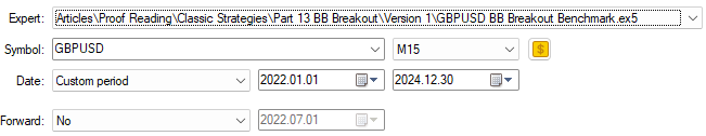
Fig 2: Selecting the time frame for our back test

Now we shall fine tune the parameters of our test. Selecting "Random delay" will see how reliable our trading system is when market conditions are unstable. Additionally, I have selected "Every tick based on real ticks" because this provides us with the most realistic simulation of past market data. In this modelling mode, our MetaTrader 5 Terminal will fetch all the real-time ticks that were sent by the broker on that day. This process can be time-consuming, depending on your internet speed. However, in the end, it is likely to yield results close to the truth.

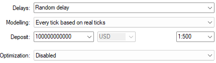
Fig 3: Selecting the back test conditions for our test

Lastly, we will define settings that will control the behavior of our application. Note, in our second test, the settings we have selected in Fig 4 will be kept constant using our system variables. Therefore, we will not be giving the second version of our application an unfair advantage over this current version we are about to test.

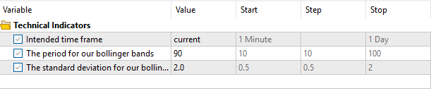
Fig 4: The input parameters for our expert advisor during this single back test

The profit curve produced by our current algorithm is inherently unstable. It unpredictably goes through periods of rapid growth, and excessive loss. The current version of our trading strategy, spent most of its time recovering from periods of drawdown, rather than accumulating profits and occasionally losing trades.  This is far from ideal. At the end of our test, our algorithm only managed to lose our capital. It is evident there is more work to be done, before we can consider using this algorithm at all. 

Fig 5: The equity curve produced by our current version of the original trading strategy

When we inspect the results of our back-test closely, we observe that our system had a healthy proportion of winning trades, 63% of all trades placed were profitable. The problem is, our profits were almost half the size of our losses. Since we do not desire to change the original trading rules, our new goal is to direct the growth in our average profit closer to its maximum while ensuring that our losing trades grow at a smaller rate. This delicate balancing act, will give us the results we desire.

Fig 6: A detailed analysis of the results produced by the original version of the trading strategy

Improving Our Initial Results

As we can see, the initial results aren't very encouraging. However, we know that the human trader who invented the Bollinger Bands and proposed these trading rules was himself a successful trader by any measure. So where is the gap between the rules created by John Bollinger, and the results we have obtained from algorithmically following his rules? 

Fig 7: The inventor of the Bollinger Bands, John Bollinger

Part of the difference may be the human application of these rules. It is likely, that over time, Bollinger developed an intuition about the market conditions under which his strategy thrives, and the conditions in which it tends to fail. Our current application constantly risks the same amount on each trade, and treats all trading opportunities equally. However, human beings can use their discretion to risk more or less, depending on their learned expectations and confidence levels about the future. 

Human traders aim to take risk when they believe it is most likely to pay off, they don't rigidly follow a given set of rules. We want to give our computer an additional level of flexibility, on top of the original strategy. Realizing this goal, may hopefully explain the gap between the results we expected, and those we have produced thus far. Therefore, we will introduce complexity, to try and bring our machine closer to what professional human beings are doing daily, as opposed to just trying to forecast future price levels directly. 

We can build a logistic regression model, to give our application a sense of "confidence". Our model's parameters will be optimized using historical market data we will fetch from our MetaTrader 5 terminal. Our native MQL5 implementation means our Expert Advisor can work on any time frame provided there is enough data on that timeframe. 

A logistic regression model is possibly the simplest model we can build today. There are many forms of logistic models, however, the form we will cover today can only be used to model 2 classes. Readers seeking to classify more than 2 classes, should consider reading more literature on logistic models.

To implement our desired changes and bring our application's decision-making process closer to the human decision-making process, we will implement a few important changes to our current version of the trading system:

Proposed Change	Intended Purpose
Additional System Constants	We will need to create new system constants to accommodate the probabilistic model we want to build, and all other new system parts we need.
Supplementary Technical Analysis	Using 2 strategies at once can unlock greater levels of profitability for our system. We will also seek confirmation from the stochastic oscillator before opening our trades to increase the probabilities of getting profitable trades.
New User Inputs	To allow our user to control the new parts of our system, we need to create new user inputs that control the new functionality we are implementing.
Modification of Custom Functions	The customized functions we have built so far need to be revised and extended to accommodate all the new variables and tasks our application is to perform

Getting Started

To get started building our revised version of the trading application, we will first need to create new system constants to keep our tests consistent across all our proposed versions of the algorithm.

//+------------------------------------------------------------------+
//|                                 GBPUSD BB Breakout Benchmark.mq5 |
//|                                               Gamuchirai Ndawana |
//|                    https://www.mql5.com/en/users/gamuchiraindawa |
//+------------------------------------------------------------------+
#property copyright "Gamuchirai Ndawana"
#property link      "https://www.mql5.com/en/users/gamuchiraindawa"
#property version   "1.00"

//+------------------------------------------------------------------+
//| System constants                                                 |
//+------------------------------------------------------------------+
#define  BB_SHIFT   0                              // Our bollinger band should not be shifted
#define  SYMBOL     "GBPUSD"                       // The intended pair for our trading system
#define  BB_PRICE   PRICE_CLOSE                    // The price our bollinger band should work on
#define  BB_PERIOD  90                             // The period for our bollinger bands
#define  BB_SD      2.0                            // The standard deviation for our bollinger bands
#define  LOT        0.1                            // Our intended lot size
#define  TF    PERIOD_M15                          // Our intended time frame
#define  ATR_MULTIPLE 20                           // ATR Multiple
#define  ATR_PERIOD 14                             // ATR Period
#define  K_PERIOD 12                               // Stochastic K period
#define  D_PERIOD 20                               // Stochastic D period
#define  STO_SMOOTHING 12                          // Stochastic smoothing
#define  LOGISTIC_MODEL_PARAMS 5                   // Total inputs to our logistic model

Additionally, we want our user to control the functionality of our logistic regression model. The "fetch" input determines how much data should be used to build our model. Note that generally speaking, the higher the time-frame the user wants to use, the less data we have. On the other hand, "look_ahead" determines how far into the future our model should attempt to forecast.

//+------------------------------------------------------------------+
//| User inputs                                                      |
//+------------------------------------------------------------------+
input int fetch = 5;                               // How many historical bars of data should we fetch?
input int look_ahead = 10;                         // How far ahead into the future should we forecast?

Moreover, we will need new global variables in our application. These variables will serve as handlers for our new technical indicators, as well as the moving parts of our logistic regression model.

//+------------------------------------------------------------------+
//| Global variables                                                 |
//+------------------------------------------------------------------+

//+------------------------------------------------------------------+
//| Technical indicators                                             |
//+------------------------------------------------------------------+
int    bb_handler,atr_handler,stoch_handler;
double bb_u[],bb_m[],bb_l[],atr[],stoch[];
double logistic_prediction;
double learning_rate = 5E-3;

vector open_price  = vector::Zeros(fetch);
vector open_price_old = vector::Zeros(fetch);
vector close_price = vector::Zeros(fetch);
vector close_price_old = vector::Zeros(fetch);
vector high_price  = vector::Zeros(fetch);
vector high_price_old = vector::Zeros(fetch);
vector low_price = vector::Zeros(fetch);
vector low_price_old = vector::Zeros(fetch);

vector target      = vector::Zeros(fetch);
vector coef        = vector::Zeros(LOGISTIC_MODEL_PARAMS);
double max_forecast = 0;
double min_forecast = 0;
double baseline_forecast = 0;

Most other parts of our trading system will remain the same, except for a few functions that need to be extended and new functions we need to define. First on the list to be edited is our initialization function. We have additional steps to perform before we are ready to start trading. We will need to set up the ATR and stochastic model, and additionally, we must define the function "setup_logistic_model()".

//+------------------------------------------------------------------+
//| Setup our technical indicators and other variables               |
//+------------------------------------------------------------------+
bool setup(void)
  {
//--- Setup our system
   bb_handler = iBands(SYMBOL,TF,BB_PERIOD,BB_SHIFT,BB_SD,BB_PRICE);
   atr_handler = iATR(SYMBOL,TF,ATR_PERIOD);
   stoch_handler = iStochastic(SYMBOL,TF,K_PERIOD,D_PERIOD,STO_SMOOTHING,MODE_EMA,STO_LOWHIGH);
   state = 0;
   higher_state = 0;
   setup_logistic_model();

//--- Validate our system has been setup correctly
   if((bb_handler != INVALID_HANDLE) && (Symbol() == SYMBOL))
      return(true);

//--- Something went wrong!
   return(false);
  }

Our logistic regression model takes a set of inputs, and predicts a probability between zero and one that the target variable will belong to the default class, given the current value of x. The model uses a sigmoid function, depicted in Fig 8 below, to calculate these odds. 

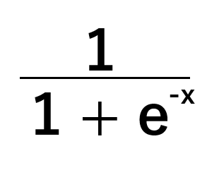
Imagine if we are interested in solving the following problem: "Given a person's weight and height, what is the probability they are male?". In this example question, being male is the default class. Probabilities above 0.5 imply the person is believed to be male, and probabilities below 0.5 imply the assumed gender to be female. This is the simplest version of the logistic model possible. There are versions of the logistic model that can classify more than 2 targets, but we will not consider them today.

The sigmoid function generalized in Fig 8 above, will transform any value of x and give us an output value between 0 and 1 as depicted in Fig 9 below.

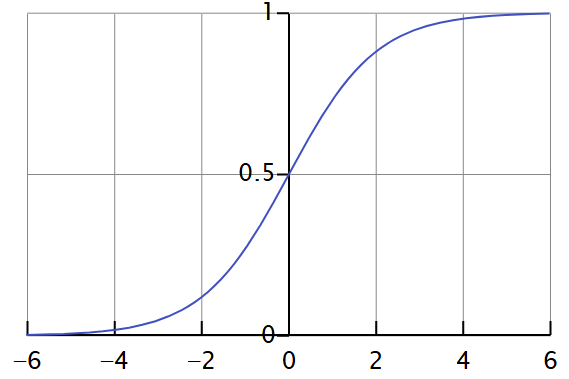
Fig 9: Visualizing the transformation of a sigmoid function

We can carefully calibrate our sigmoid function so that it produces estimates close to 1 for all the observations in our training data that belonged to class 1 and likewise estimates close to 0 for all values in our training data that belonged to class 0. This algorithm is known as maximum likelihood estimation. We can approximate these results using a much simpler algorithm known as gradient descent. 

In the code provided below, we begin by first preparing our input data. We find the change in the open, high, low and close price, these will be our inputs for the model. Afterward, we record the associated future change in price. If price levels fell, we will record this as class 0. Class 0 is our default class. Predictions above our cutoff point, imply that our model expects future price levels to fall. Likewise, predictions below the cut-off point, imply that the default class is not true, or in our case, our model expects price levels to rise. Typically, a cut-off point of 0.5 is preferred.

After labelling our data, we initialize all our model coefficients to 0, and then proceed to make the first prediction with these poor coefficients. With each prediction, we correct the coefficients using the difference between our prediction and the true label. This process is repeated for each bar we fetched. 

Lastly, I stated earlier that a cutoff point of 0.5 is classically preferred. However, financial markets are not well known for being well-behaved environments. The classical approach did not yield probabilities useful for us as traders, so I extended the classical algorithm and calibrated it even further.

I included an additional step to calculate an optimal cutoff point by first recording the maximum and minimum odds forecasted by our model. We then bisected the true range of predictions given by our model to find our cutoff point. Given the financial market can be noisy, it may be challenging for our models to learn effectively, and we may need to get creative and find new ways of interpreting our models. This dynamic cutoff point will help our model make its decisions independent of our inherent bias.

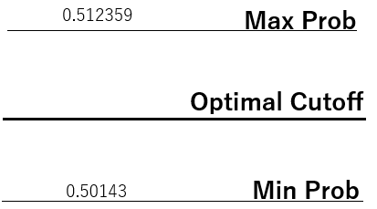
Fig 10: Visualizing how we dynamically set our cutoff point

So in our case, probabilities above our dynamic cutoff point will be interpreted as the default class, meaning our model believes we should "sell". And the opposite is true for predictions that lie below our dynamic cutoff point.

//+------------------------------------------------------------------+
//| Setup our logistic regression model                              |
//+------------------------------------------------------------------+
void setup_logistic_model(void)
  {
   open_price.CopyRates(SYMBOL,TF,COPY_RATES_OPEN,(fetch + look_ahead),fetch);
   open_price_old.CopyRates(SYMBOL,TF,COPY_RATES_OPEN,(fetch + (look_ahead * 2)),fetch);

   high_price.CopyRates(SYMBOL,TF,COPY_RATES_HIGH,(fetch + look_ahead),fetch);
   high_price_old.CopyRates(SYMBOL,TF,COPY_RATES_HIGH,(fetch + (look_ahead * 2)),fetch);

   low_price.CopyRates(SYMBOL,TF,COPY_RATES_LOW,(fetch + look_ahead),fetch);
   low_price_old.CopyRates(SYMBOL,TF,COPY_RATES_LOW,(fetch + (look_ahead * 2)),fetch);

   close_price.CopyRates(SYMBOL,TF,COPY_RATES_CLOSE,(fetch + look_ahead),fetch);
   close_price_old.CopyRates(SYMBOL,TF,COPY_RATES_CLOSE,(fetch + (look_ahead * 2)),fetch);

   open_price = open_price - open_price_old;
   high_price = high_price - high_price_old;
   low_price = low_price - low_price_old;
   close_price = close_price - close_price_old;

   CopyBuffer(atr_handler,0,0,fetch,atr);

   for(int i = (fetch + look_ahead); i > look_ahead; i--)
     {
      if(iClose(SYMBOL,TF,i) > iClose(SYMBOL,TF,i - look_ahead))
         target[i-look_ahead-1] = 0;
      if(iClose(SYMBOL,TF,i) < iClose(SYMBOL,TF,i - look_ahead))
         target[i-look_ahead-1] = 1;
     }

//Fitting our coefficients
   coef[0] = 0;
   coef[1] = 0;
   coef[2] = 0;
   coef[3] = 0;
   coef[4] = 0;

   for(int i =0; i < fetch; i++)
     {
      double prediction = 1 / (1 + MathExp(-(coef[0] + (coef[1] * open_price[i]) + (coef[2] * high_price[i]) + (coef[3] * low_price[i]) + (coef[4] * close_price[i]))));
      coef[0] = coef[0] + (learning_rate * (target[i] - prediction)) * prediction * (1 - prediction) * 1.0;
      coef[1] = coef[1] + (learning_rate * (target[i] - prediction)) * prediction * (1 - prediction) * open_price[i];
      coef[2] = coef[2] + (learning_rate * (target[i] - prediction)) * prediction * (1 - prediction) * high_price[i];
      coef[3] = coef[3] + (learning_rate * (target[i] - prediction)) * prediction * (1 - prediction) * low_price[i];
      coef[4] = coef[4] + (learning_rate * (target[i] - prediction)) * prediction * (1 - prediction) * close_price[i];
     }

   for(int i =0; i < fetch; i++)
     {
      double prediction = 1 / (1 + MathExp(-(coef[0] + (coef[1] * open_price[i]) + (coef[2] * high_price[i]) + (coef[3] * low_price[i]) + (coef[4] * close_price[i]))));
      if(i == 0)
        {
         max_forecast = prediction;
         min_forecast = prediction;
        }
      max_forecast = (prediction > max_forecast) ? (prediction) : max_forecast;
      min_forecast = (prediction < min_forecast) ? (prediction) : min_forecast;
     }

   baseline_forecast = ((max_forecast + min_forecast) / 2);

   Print(coef);
   Print("Baseline: ",baseline_forecast);
  }

If we aren't using our Expert Advisor, there are a few additional technical indicators we need to release.

//+------------------------------------------------------------------+
//| Release the resources we no longer need                          |
//+------------------------------------------------------------------+
void release(void)
  {
//--- Free up system resources for our end user
   IndicatorRelease(bb_handler);
   IndicatorRelease(atr_handler);
   IndicatorRelease(stoch_handler);
  }

Our conditions for setting up positions remain mostly the same, except if our model's predictions align with the trading rules proposed by John Bollinger, we will double down on that opportunity and instruct our application to take on more risk only under those conditions.

//+------------------------------------------------------------------+
//| Find an oppurtunity to trade                                     |
//+------------------------------------------------------------------+
void find_setup(void)
  {
   double open_input = iOpen(SYMBOL,TF,0)   - iOpen(SYMBOL,TF,look_ahead);
   double close_input = iClose(SYMBOL,TF,0) - iClose(SYMBOL,TF,look_ahead);
   double high_input = iHigh(SYMBOL,TF,0)   - iHigh(SYMBOL,TF,look_ahead);
   double low_input = iLow(SYMBOL,TF,0)     - iLow(SYMBOL,TF,look_ahead);
   double prediction = 1 / (1 + MathExp(-(coef[0] + (coef[1] * open_input) + (coef[2] * high_input) + (coef[3] * low_input) + (coef[4] * close_input))));
   Print("Odds: ",prediction - baseline_forecast);
   
//--- Check if we have breached the bollinger bands
   if((c > bb_u[0]) && (stoch[0] < 50))
     {
      
      Trade.Sell(LOT,SYMBOL,bid);
      state = -1;

      if(((prediction - baseline_forecast) > 0))
        {
         Trade.Sell((LOT * 2),SYMBOL,bid);
         Trade.Sell((LOT * 2),SYMBOL,bid);
         state = -1;
        }

      return;
     }

   if((c < bb_l[0]) && (stoch[0] > 50))
     {
      
      Trade.Buy(LOT,SYMBOL,ask);
      state = 1;
      
      if(((prediction - baseline_forecast) < 0))
        {
         Trade.Buy((LOT * 2),SYMBOL,ask);
         Trade.Buy((LOT * 2),SYMBOL,ask);
         state = 1;
        }

      return;
     }
  }

Additionally, we want to have a stop loss that will trail if our trade is winning, and otherwise it should stay put. This will ensure that we reduce our risk if we are winning, which is a smart thing human traders do all the time.

//+------------------------------------------------------------------+
//| Manage our open positions                                        |
//+------------------------------------------------------------------+
void manage_setup(void)
  {
   if(((c < bb_l[0]) && (state == -1))||((c > bb_u[0]) && (state == 1)))
      Trade.PositionClose(SYMBOL);


//--- Update the stop loss
   for(int i = PositionsTotal() -1; i >= 0; i--)
     {
      string symbol = PositionGetSymbol(i);
      if(_Symbol == symbol)
        {
         double position_size = PositionGetDouble(POSITION_VOLUME);
         double risk_factor = 1;
         if(position_size == (LOT * 2))
            risk_factor = 2;
         double atr_stop = atr[0] * ATR_MULTIPLE * risk_factor;
         ulong ticket = PositionGetInteger(POSITION_TICKET);
         double position_price = PositionGetDouble(POSITION_PRICE_OPEN);
         long type = PositionGetInteger(POSITION_TYPE);
         double current_take_profit = PositionGetDouble(POSITION_TP);
         double current_stop_loss = PositionGetDouble(POSITION_SL);
         if(type == POSITION_TYPE_BUY)
           {
            double atr_stop_loss = (bid - (atr_stop));
            double atr_take_profit = (bid + (atr_stop));

            if((current_stop_loss < atr_stop_loss) || (current_stop_loss == 0))
              {
               Trade.PositionModify(ticket,atr_stop_loss,current_take_profit);
              }
           }
         else+
            if(type == POSITION_TYPE_SELL)
              {
               double atr_stop_loss = (ask + (atr_stop));
               double atr_take_profit = (ask - (atr_stop));
               if((current_stop_loss > atr_stop_loss) || (current_stop_loss == 0))
                 {
                  Trade.PositionModify(ticket,atr_stop_loss,current_take_profit);
                 }
              }
        }
     }
  }
//+------------------------------------------------------------------+

The settings controlling the duration and time-frame of the back-test will be kept the same, the only variable we must change here is the Expert being selected. We have selected the revised version of the application that we have just refactored together in the previous section of this article. Ensure that you also keep your settings the same, while you select the new version of the application.

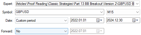
Fig 11: Selecting the time-frame and period for our second back-test to evaluate the effectiveness of our chosen settings

As always, be sure to select leverage settings that match your agreement with your broker. Incorrectly specifying your leverage settings, may give you unrealistic expectations about the profitability of your trading applications. To make matters worse, you may find it challenging to reproduce the results you obtain in your back-test, especially if the leverage settings in your real account do not match the leverage settings you are using in your back-test. This is a commonly overlooked source of error when performing back-tests, so take your time.

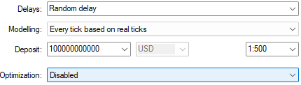
Fig 12: Back-tests are sensitive to the settings selected when launching the back-test. Ensure you get it right the first time

Now we shall define how much data our trading application should fetch to estimate the parameters of our logistic regression model, and the forecast horizon for our model. Do not try and fetch more data than what your broker provides to you. Otherwise, the application will not work as intended! Also, set a forecast horizon that is inline with your risk tolerance.

For example, you may wish to train your application to look ahead 2000 steps in the future. However, you must bear in mind that 2000 steps into the future on the M15 time frame corresponds to about 20 days. If you, as a human, do not realistically forecast this far ahead into the future when you are placing your trades, then do not try to force the application to do so. Recall that our goal is to build an application that emulates what you do every day, as a human trader.

Fig 13: The parameters controlling the behavior of our trading application and our logistic regression model

Now we have arrived at the most informative part of our test. Our new system produced an average profit of $79. Initially, we expected an average profit of $45. Therefore, the difference between our current expected profit ($79) and our previous expected profit ($45) is $34. This $34 difference, corresponds to a growth of approximately 75% of the original expected profit.

Simultaneously, our new expected loss is $-122, while our initial expected loss was $-81. This is a difference of $41, and corresponds to an approximately 50% growth in the size of our average loss. So we have successfully achieved our goal!

Our new settings, ensure that our profits are growing at a larger rate, than our losses. This is also the reason we successfully rectified our Sharpe ratio and expected payoff. Our initial version of the trading strategy accumulated a loss of $-791, while our new system accumulated a profit of $2 274 without changing the rules of the algorithm or the period of the back-test.

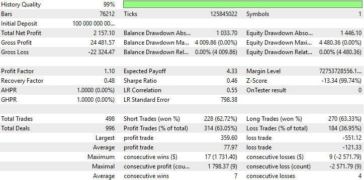
Fig 14: Ideally, we would want our losses to have a growth rate of 0, but the real world is not ideal

When we now observe the equity curve our algorithm produces, we can clearly see that our algorithm is more stable than it was initially. All trading strategies will go through periods of drawdown. However, we are interested in the ability of the strategy to recover from loss and preserve its profits eventually. A strategy that is too risk-adverse, may hardly make any profit and on the contrary, a strategy that has a strong affinity for risk, may quickly lose all the profits it makes. Therefore, we have managed to strike a balance, in the middle.

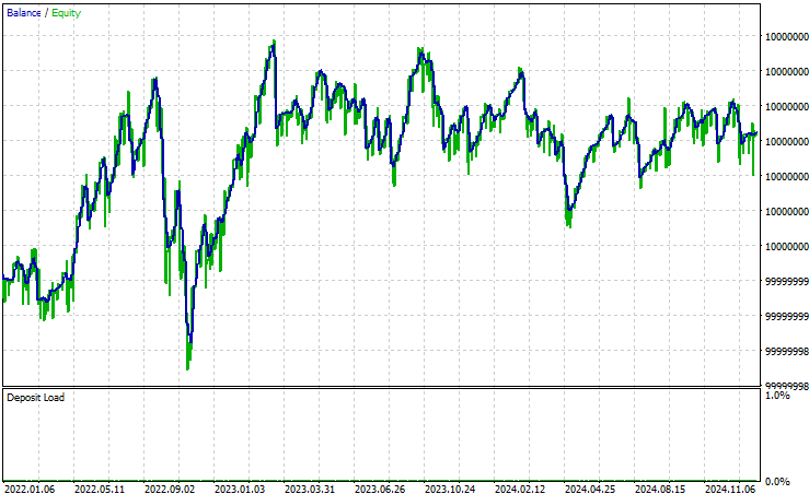
Fig 15: The equity curve produced by our new version of the trading algorithm is more desirable than our initial results

Conclusion

Controlling the amount of risk being taken by our trading applications is pivotal to ensure profitable and sustainable trading. This article has demonstrated how you can design your applications to independently increase the lot size if our application detects that our trade has a high chance of being profitable. Otherwise, if our expectation is that the trade may not work out, our application will risk the smallest amount possible. This dynamic position sizing is crucial for profitable trading because it ensures we are making the most out of each opportunity we have, and managing our risk levels responsibly. By building a probabilistic logistic model together, we have learned one possible way of insuring that our application is selecting the optimal position size, based on what it has learned about the market at hand.

Attached File	Description
GBPUSD BB Breakout Benchmark	This is the initial version of our trading application, and was not profitable on our first test.
GBPUSD BB Breakout Benchmark V2	The refined algorithm based on the same trading rules, but designed to take intelligently increase our position sizes if it detects we have a good chance of winning.