Recipes for Neuronets

Introduction

Not so long ago - at the dawn of technical analysis when by far not all traders had computers - people appeared that tried to predict future prices using formulas and regularities invented by them. They were often called charlatans. Time went on, methods of information processing became more complicated, and now there can hardly be traders indifferent to technical analysis. Any beginning trader can easily utilize charts, various indicators, search for regularities.

The number of forex-traders grows daily. Together with that their requirements for market analyzing methods grow. One of such "relatively" new methods is the use of theoretically fuzzy logics and neural networks. We see that topics devoted to these questions are being actively discussed on various thematic forums. They do exist, and will go on existing. A human that entered the market will hardly ever leave it. While it is the challenge to one's intelligence, brain and strength of will. That is why a trader never ceases to study something new and to use various approaches in practice.

In this article we will analyze basics of neuronet creation, will learn about the notion of Kohonen neural net and will talk a little about methods of trading optimization. This article is first of all intended for traders who are only at their beginning in studying neuronets and principles of information processing.

To cook a neural network with the Kohonen layer one would need:

1) 10 000 history bars of any currency pair;
2) 5 grams of moving averages (or any other indicators - it is up to you);
3) 2-3 layers of inverse distribution;
4) methods of optimization as its stuffing;
5) the greens of growing balance and number of correctly guessed trade directions.

Section I. Recipe of the Kohonen Layer

Let's start with the section for those who are at the very start. We will discuss various approaches to the training of the Kohonen layer or, to be more exact, its basic version, because there are many variants of it. There is nothing original about this chapter, all explanations are taken from classical references on this theme. However, the advantage of this chapter is the large number of explanatory pictures for each section.

In this chapter we will dwell on the following questions:
- the way Kohonen weight vectors are adjusted;
- preliminary preparation of input vectors;
- selection of initial weights of Kohonen neurons.

So, as per Wikipedia, Kohonen neural network represents a class of neural networks, the main element of which is the Kohonen layer. The Kohonen layer consists of adaptive linear adders ("linear formal neurons"). As a rule, output signals of the Kohonen layer are processed according to the rule "the winner takes it all": the largest signals turn into one, all other signals turn into zeros.

Now let's discuss this notion on an example. For the purpose of visualization all calculations will be given for two-dimensional input vectors. In fig. 1 the input vector is shown in color. Each neuron of the Kohonen layer (as of any other layer) simply sums up the input, multiplying it by its weights. Actually, all weights of the Kohonen layer are vector coordinates for this neuron.

Thus, output of each Kohonen neuron is the dot product of two vectors. From geometry we know that the maximal dot product will be if the angle between vectors tends to zero (the angle cosine tends to 1).So, the maximal value will be that of the Kohonen layer neuron that is the closest to the input vector.

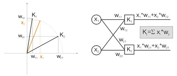
Fig.1 The winner is the neuron whose vector is the closest to the input signal.

As per the definition, now we should find the maximal output value among all neurons, assign its output to one and assign zero to all other neurons. And the Kohonen layer will "reply" to us in which space area the input vector lies.

Adjustment of Kohonen Weight Vectors

The purpose of layer training, as written above, is the precise space classification of input vectors. This means that each neuron must be responsible for its certain area, in which it is the winner. The deviation error of the winner-neuron from the input neuron must be smaller than that of other neurons. To achieve it the winner neuron "turns" in the side of the input vector.
Fig 2 shows the division of two neurons (black neurons) for two input vectors (colored ones).

Fig.2. Each of neurons approaches its nearest input signal.

With each iteration, the winner neuron approaches "its own" input vector. Its new coordinates are calculated according to the following formula:

where A(t) is the parameter of training speed, depending on the time t. This is a nonincreasing function that is reduced at each iteration from 1 to 0. If the initial value is A=1, the weight correction is made at one stage. This is possible when for each input vector there is one Kohonen neuron (for example, 10 input vectors and 10 neurons in Kohonen layer).

But in practice such cases are almost never met, because usually the large volume of input data needs to be divided into groups of similar ones, thus diminishing the diversity of input data. That is why the value A=1 is undesirable. Practice shows that the optimal initial value should be below 0.3.

Besides, A is inversely proportional to the number of input vectors. I.e. at a large selection it is better to make small corrections, so that the winner neuron does not "surf" through the whole space in its corrections. As the A functionality usually any monotonically decreasing function is chosen. For example, hyperbola or linear decrease, or Gaussian function.
Fig. 3 shows the step of neuron weights correction at the speed A=0.5. The neuron has neared the input vector, the error is smaller.

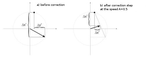
Fig.3. Neuron weights correction under the influence of the input signal.

Small Number of Neurons at a Wide Sample

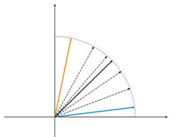
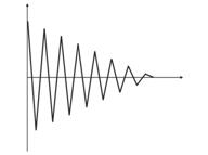
Fig.4. Neuron fluctuations between two input vectors.

In fig. 4 (left) there are two input vectors (shown in color) and only one Kohonen neuron. In the process of correction the neuron will swing from one vector to another (dotted lines). As the A value diminishes till 0 it stabilizes between them. Neuron coordinate changes from time can be characterized by a zigzag line (fig. 4 right).

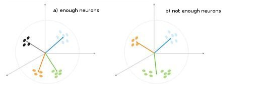
Fig. 5. Dependence of the classification type on the number of neurons.

One more situation is shown in fig. 5. In the first case four neurons adequately divide the sample into four areas of hypersphere. In the second case the insufficient number of neurons result in the increased error and re-classification of the sample. Thus we can conclude that the Kohonen layer must contain the sufficient number of free neurons which depends on the volume of the classified sample.

Preliminary Preparations if Input Vectors
As Philip D. Wasserman writes in his book, it is desirable (though not obligatory) to normalize input vectors before you introduce them to the net. This is done by dividing each component of the input vector by the vector length. This length is found by the extraction of a square root from the sum of squares of vector components. This is the algebraic presentation:

This transforms the input vector into a unit vector with the same direction, i.e. a vector with the unit length in the n-dimension space. The meaning of this operation is clear - projecting all input vectors on the hypersphere surface, thus simplifying the task of searching to the Kohonen layer. In other words, for we are searching for the angle between input vectors and vectors-Kohonen neurons, we should eliminate such a factor as the vector length, equating chances of all neurons.

Very often elements of sample vectors are non-negative values (for example, values of moving averages, price). All they are concentrated in the positive quadrant space. As the result of normalization of such a "positive" sample we obtain the large accumulation of vectors in only one positive area, which is not very good for the qualification. That is why prior to normalization the sample smoothing can be performed. If the sample is rather large, we can assume that vectors are located approximately in one area without "outsiders" which are far away from the main sample. Therefore, a sample can be centered relative to its "extreme" coordinates.

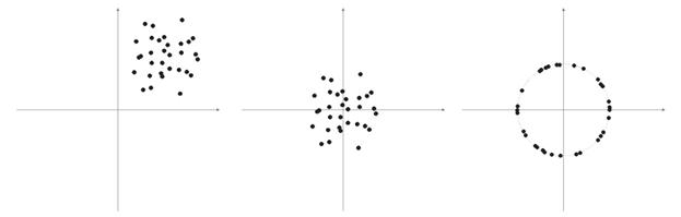
Fig. 6. Normalization of input vectors.

As written above, normalization of vectors is desirable. It simplifies the correction of the Kohonen layer. However we should clearly represent a sample and decide whether it should be projected on a sphere or not.

Listing 1. Narrowing of input vectors into the range [-1, 1]

for (N=0; N<nNeuron[0]; N++) // for all neurons of the input layer
 {
  min=in[N][0]; // finding minimum in the whole sample
  for (pat=0; pat<nPattern; pat++) if (in[N][pat]<min) min=in[N][pat];
  for (pat=0; pat<nPattern; pat++) in[N][pat]-=min; // shift by the value of the minimal value 
  max=in[N][0]; // finding maximum in the whole sample
  for (pat=0; pat<nPattern; pat++) if (in[N][pat]>max) max=in[N][pat];
  for (pat=0; pat<nPattern; pat++) in[N][pat]=2*(in[N][pat]/max)-1; // narrowing till [-1,1]
 }

If we normalize input vectors, we should correspondingly normalize all neuron weights.


Selecting Initial Neuron Weights
Possible variants are numerous.
1) Random values are assigned to weights, as is usual done with neurons (randomizing);
2) Initialization by examples, when values of randomly selected examples from a training sample are assigned as initial values;
3) Linear initialization. In this case weights are initiated by vector values that are linearly ordered along the whole linear space located between two vectors from the initial set of data;
4) All weights have the same value - method of convex combination.

Let's analyze the first and the last cases.
1) Random values are assigned to weights.

During randomization all vector-neurons are distributed upon the surface of a hypersphere. While input vectors have a tendency of grouping. In this case it may happen that some weight vectors are so much distanced from input vectors that they will never be able to give a better correlation and, consequently, will not be able to learn - "grey" figures in fig. 7 (right). Moreover, the remaining neurons will not be enough for minimizing the error and divide similar classes - the "red" class is included into the "green" neuron.

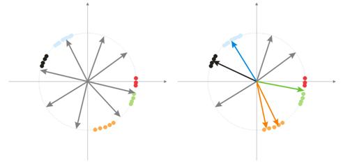
Fig. 7. Training result of randomized neurons.

And if there is a large accumulation of neurons in one area, several neurons can enter the area of one class and divide it into sub-classes - orange area in fig. 7. This is not critical, because further processing of layer signals can fix the situation but this takes the training time.

One of variants for solving these problems is the method when at initial stages correction is made not only for vectors of one winning neuron, but for the group of vectors closest to it as well. Then the number of the group diminishes gradually and finally only one neuron is corrected. A group can be selected from a sorted array of neuron outputs. Neurons from first K maximal outputs will be corrected.

One more approach in the group adjustment of weight vectors is the following method.

a) For each neuron the length of correction vector is defined:

.
b) A neuron with the minimal distance becomes a winner – Wn. After that a group of neurons if found, correlation of which is in limits of distance C*Ln from Wn.
c) Weights of these neurons are corrected by a simple rule . Thus the correction of the whole sample is made.

The C parameter changes in the process of training from some number (usually from 1) to 0.

The third interesting method implies that each neuron can be corrected only N/k times for one passing through the sample. Here N is the size of the sample, k- the number of neurons. I.e. if any of neurons becomes a winner oftener than others, it "quits the game" till the end of passing through the sample. Thus other neurons can learn as well.

2) method of convex combination

The meaning of the method implies that both weight and input vectors are initially placed in one area. Calculation formulas for current coordinates of input and initial weight vectors will be the following:

,

where n is the dimension of an input vector, a(t)- non-decreasing function on time, with each iteration increases its value from 0 to 1, as a result of which all input vectors coincide with weight vectors and finally take their places. Besides, weight vectors will be "reaching" for their classes.

This is all material on the basic version of the Kohonen layer that will be applied in this neural network.

II. Spoons, Ladles and Scripts

The first script that we are going to discuss will gather data on bars and create a file of input vectors. As a training example let's use MA.

Listing 2. Creating a file of input vectors

// input parameters
 #define NUM_BAR 10000 // number of bars for training (number of training patterns)
 #define NUM_MA 5 // number of movings
 #define DEPTH_MA 3 // number of values of a moving
 // creating a file
 hFile = FileOpen(FileName, FILE_WRITE|FILE_CSV);
 FileSeek(hFile, 0, SEEK_END); 
 // Creating an array of inputs
 int i, ma, depth;
 double MaIn;
 for (i=NUM_BAR; i>0; i--) // going through bars and collecting values of MA fan 
 {
  for (depth=0; depth<DEPTH_MA; depth++) //calculating moving values
   for (ma=0; ma<NUM_MA; ma++) 
   {
   MaIn=iMA(NULL, 0, 2+MathSqrt(ma*ma*ma)*3, 0, 1, 4, 
                    i+depth*depth)- ((High[i+depth*depth] + Low[i+depth*depth])/2);
   FileWriteDouble(hFile, MaIn);
   }
  }

The data file is created as the means for transmitting information between applications. When you are getting acquainted with training algorithms, it is strongly recommended to watch the interim results of their operation, values of some variables and, if necessary, change training conditions.

That is why we recommend you to use the programming language of a high level (VB, VC++ etc.), while currently debugging means of MQL4 are not enough (I hope this situation will be improved in MQL5). Later, when you learn all the pitfalls of your algorithms and functions, you can start using MQL4. Besides, you will have to write the final target (indicator or Expert Advisor) in MQL4.

Generalized Structure of Classes

Listing 3. Class of neural network

class CNeuroNet : public CObject  
 {
 public:
  int nCycle; // number of learning cycles until stop
  int nPattern; // number of training patterns
  int nLayer; // number of training layers
  double Delta; // required minimal output error
  int nNeuron[iMaxLayer]; // number of neurons in a layer (by layers)
  int LayerType[iMaxLayer]; // types of layers (by layers)
  double W[iMaxLayer][iMaxNeuron][iMaxNeuron];// weights by layers
  double dW[iMaxLayer][iMaxNeuron][iMaxNeuron];// correction of weight
  double Thresh[iMaxLayer][iMaxNeuron]; // threshold
  double dThresh[iMaxLayer][iMaxNeuron]; // correction of threshold
  double Out[iMaxLayer][iMaxNeuron]; // output value
  double OutArr[iMaxNeuron]; // sorted output values of Kohonen layer
  int IndexWin[iMaxNeuron]; // sorted neuron indexes of Kohonen layer
  double Err[iMaxLayer][iMaxNeuron][iMaxNeuron];// error

  double Speed; // Speed of training
  double Impuls; // Impulse of training

  double in[100][iMaxPattern]; // Vector of input values
  double out[10][iMaxPattern]; // vector of output values
  double pout[10]; // previous vector of output values
  double bar[4][iMaxPattern]; // bars, on which we learn
  int TradePos; // order direction
  double ProfitPos; // obtained profit/loss of an order

 public:
  CNeuroNet();
  virtual ~CNeuroNet();
  // functions
  void Init(int aPattern=1, int aLayer=1, int aCycle=10000, double aDelta=0.01, double aSpeed=0.1, 
                                                                               double aImpuls=0.1);
  // learning functions
  void CalculateLayer(); // Calculation of layer output
  void CalculateError(); // Error calculation /for Target array/
  void ChangeWeight(); // Correction of weights
  bool TrainNetwork(); // Network training
  void CalculateLayer(int L); // Output calculation of Kohonen layer
  void CalculateError(int L); // Error calculation of Kohonen layer
  void ChangeWeight(int L); // Correction of weights for layer indication
  bool TrainNetwork(int L); // Training of Kohonen layer

  bool TrainMPS(); // Network training for getting the best profit

  // variables for internal interchange
  bool bInProc; // flag for entering the TrainNetwork function
  bool bStop; // flag for the forced termination of the TrainNetwork function
  int loop; // number of the current iteration
  int pat; // number of the current processed pattern
  int iMaxErr; // pattern with the maximal error
  double dMaxErr; // maximal error
  double sErr; // square of pattern error
  int iNeuron; // maximal number of neurons in Kohonen layer correction
  int iWinNeuron; // number of winner neurons in Kohonen layer

  int WinNeuron[iMaxNeuron]; // array of active neurons (ordered)
  int NeuroPat[iMaxPattern][iMaxNeuron]; // array of active neurons

  void LinearCovariation(); // normalization of the sample
  void SaveW(); // Analysis of neuron activity
 };

Actually the class is not complex. It contains the main necessary set + service variables.

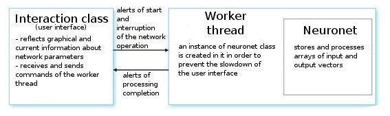
Let's analyze it. Upon a user's command, the interface class creates a work thread and initializes a timer for the periodical readout of the network values. It also receives indexes for reading information from neuronet parameters. The worker thread in its turn first reads arrays of input/output vectors from the preliminarily prepared file and sets parameters for layers (types of layers and number of neurons in each layer). This is the preparation stage.

After that we call the function CNeuroNet::Init, in which weights are initialized, sample is normalized and training parameters are set (speed, impulse, required error and number of training cycles). And only after that we call the "workhorse" - CNeuroNet::TrainNetwork function (or TrainMPS, or TrainNetwork(int L), depending on what we want to obtain). When the training is over, the worker thread saves the network weights into a file for the implementation of the last one in an indicator or Expert Advisor.

III. Baking the Network

Now let's go to issues of training. The usual practice in training is setting the pair "pattern-teacher". That is a certain target corresponds to each input pattern. On the basis of the difference between the current input and the target value correction of weights is performed. For example, a researcher wants the net to predict the price of the following bar on the basis of prices of previous 10 bars presented to the net. In this case after placing for the input 10 values we need to compare the obtained output and the teacher value and then correct weights for the difference between them.

In the model that we offer, there will be no "teaching" vectors in the usual sense because we do not know beforehand on what bars we should enter or exit the market. It means that our network will correct its output vectors based on its own previous output values. It means the network will try to get the maximal profit (maximization of the number of correctly predicted trade directions). Let's consider an example at fig. 8.

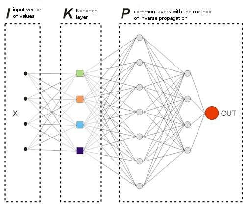
Fig. 8. Scheme of a trained neural network.

The Kohonen layer that is pre-trained on a sample forwards its vector further to the network. At the output of the last layer of the network we will have the value OUT, which is interpreted the following way. If OUT>0.5, enter a Buy; if OUT<0.5, enter a Sell (the sigmoid values are changed in limits [0, 1]).

Suppose to some input vector X1 the network replied by the output OUT1>0.5. It means on the bar to which the pattern belongs we open a Buy position. After that, at the chronological presentation of input vectors on some Xk the sign OUTk turns into the "opposite". Consequently, we close the Buy position and open a Sell position.

Exactly at this moment we need to view the result of the closed order. If we obtain profit, we can strengthen this alert. Or we can consider there is no error and will not correct anything. If we get losses, we correct the weights of layers in such a manner that the entering by the alert of X1 vector shows OUT1<0.5.

Now let's calculate the value of a teacher (target) output. As such let's take the value of a sigmoid from the obtained loss (in points) multiplied by the sign of trade direction. Consequently, the larger the loss, the stricter the network will be punished and will correct its weights by the larger value. For example, if we have =50 loss points at Buy, the correction for the output layer will be calculated as shown below:

, ,

We can delimit trading rules introducing into the trade analyzing process parameters of TakeProfit (TP) and StopLoss (SL) in points. So we need to trace 3 events: 1) change of the OUT sign, 2) price changes from the open price by the value of TP, 3) price changes from the open price by the value -SL.

When one of these events happens, the correction of weights is performed in the analogous way. If we obtain profit, weights either remain unchanged or are corrected (stronger signal). If we have loss, weights are corrected to make the input by the alert of X1 vector show OUT1 with the "desired" sign.

The only disadvantage of this limitation is the fact that we use absolute TP and SL values which is not so good for the optimization of a network on a long time period in current market conditions. As per my notice, TP and SL should not differ much from each other.

It means the system must be symmetrical in order to avoid deviation in the direction of a more global Buy or Sell trend during training. There is also an opinion that TP should be 2-4 times larger than SL - thus we artificially increase the ratio of profitable and losing trades. But in such a case we risk training the network with a shift towards trend. Of course, these two variants can exist, but you should check both of them in your investigations.

Listing 4. One iteration of network weight setup

int TradePos;
 int pat=0; // open an order for the first pattern
 for(i=0;i<nNeuron[0];i++) Out[0][i]=in[i][pat]; // take the training pattern
 CalculateLayer(); // calculate the network output
 TradePos=TradeDir(Out[nLayer-1][0]); // if exit is larger than 0.5, then buy. Otherwise - sell
 ipat=pat; // remember the pattern
 for(pat=1;pat<nPattern;pat++) // go through the pattern and train the network
 {
  for(i=0;i<nNeuron[0];i++) Out[0][i]=in[i][pat]; // take the training pattern
  CalculateLayer(); // calculate the network output
  ProfitPos=1e4*TradePos*(bar[3][pat]-bar[3][ipat]); // calculate profit/loss at close prices [3]
  // if trade direction has changed or stop order has triggered
  if (TradeDir(Out[nLayer-1][0])!=TradePos || ProfitPos>=TP || ProfitPos<=-SL) 
  {
   // correcting weights
   Out[nLayer][0]=Sigmoid(0.1*TradePos*ProfitPos); // set the desired output of the network
   for(i=0;i<nNeuron[0];i++) Out[0][i]=in[i][ipat];// take the pattern by which
                                                   // CalculateLayer() were opened;  
                                                   // calculate the network output
   CalculateError(); // calculate the error
   ChangeWeight(); // correct weights
   for(i=0;i<nNeuron[0];i++) Out[0][i]=in[i][pat]; // go to the new order CalculateLayer(); 
                                                   // calculate the new output of the network
   TradePos=TradeDir(Out[nLayer-1][0]);            // if output is > 0.5, then buy 
                                                   //otherwise sell ipat=pat; 
                                                   // remember the pattern
  }
 }

By these simple passes the network will finally distribute obtained classes from the Kohonen layer in such a manner that there is an alert of market entering with the maximal number of profits corresponding to each of them. From the point of view of statistics - each input pattern is adjusted by the net for the group work.

While one and the same input vector can give alerts in different directions during the process of weight adjustment, gradually obtaining the maximal number of true predictions, this method can be called dynamic. The method used is known as MPS - Profit-Maximizing System.

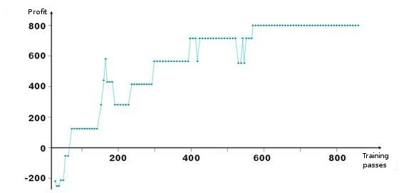
Here are results of network weights adjustment. Each point on the graph is the value of the obtained profit in points during one passing of the training period. The system is always in the market, TakeProfit = StopLoss = 50 points, fixing is made only by a stop order, weights are corrected in case of profit and loss.

See, after the negative start weights of layers are adjusted so that on the about hundredth iteration the profit becomes positive. Interesting is the fact that the system a kind of slows down at some levels. This is connected with parameters of training speed.

As you can see in the listing 2, the profit ProfitPos is calculated by close prices of a bar, on which we entered, and on which one of conditions was met (stop order or alert change). Of course, this is a rough method, especially for the case with stop orders. We can add a complication by analyzing High and Low prices of a bar (bar[1][ipat] and bar[2][ipat] correspondingly). You can try to do it yourself.

Turn or Search for Entries?
So, we studied the dynamic method of training that trains the network by its own mistakes. You must have noticed that according to the algorithm we are always in the market, fix profit/loss and go further. So, we need to delimit our entries and try to enter the market only at "favorable" input vectors. It means we need to define the dependence of the entering network alert level on the number of profitable/losing trades.

It can be done quite easily. Let's introduce the variable 0<M<0.5 that will be the criterion of an entrance needed. Of Out>0.5+M, then buy, if Out<0.5-M, then sell. We sift out entries and exits on those vectors that lie between 0.5-M<Out<0.5+M.

Another method for sifting out unnecessary vectors is gathering of statistical information about the profitability of an order from values of certain outputs of the network. Let's call it visual analysis. Before that we should define the method of position closing - stop order hitting, network output sign change. Then let's create a table Out | ProfitPos. Values of Out and ProfitPos are calculated for each input vector (i.e. for each bar).

Then let's make the summary table of the ProfitPos field. As the result we will see the dependence of the Out value and profit obtained. Select the range Out=[MLo, MHi], in which we have the best profit and use its values in trading.

Back to MQL4
Having started the development in VC++, we didn't try to depreciate the possibilities of MQL4. This was for the sake of convenience. I will tell you about an incidence. Recently one of my acquaintances tried to get a base of companies of our city. There are a lot of directories in the Internet, but no one wanted to sell the base.

And we wrote a script in MQL4 that scans an html page and selects an area with information about a company, then saving it into a file. Then we edited the file in Excel and the data base of three large yellow pages with all telephone numbers, addresses and company activities was ready. This was the most complete database in the city; for me it was the feeling of pride for easiness and possibilities of MQL4.

Naturally, one can handle one and the same task in different languages, but it is better to select the one that will be optimal in terms of possibility/difficulty ratio for a certain task.

So, after network training we should save all its parameters into a file for transferring it into MQL4.
- size of input vector
- size of output vector
- number of layers
- number of neurons by layers - from input to output
- weights of neurons by layers
The indicator will use only one function from the arsenal of the class CNeuroNet – CalculateLayer. Let's form an input vector for each bar, calculate value of the network output and build the indicator [6].

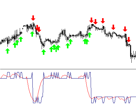
If we have already decided on input levels, we can paint parts of the obtained curve in different colors.
Example of the code !NeuroInd.mq4 is attached to the article.

IV. Creative Approach

For a good implementation we should have a wide mind. Neural networks are not the exception. I do not think the offered variant is ideal and can suit any task. That is why you should always search for your own solutions, draw the general picture, systematize and check ideas. Below you will find a few warnings and recommendations.
- Network adaptation. A neural network is an approximator. A neuronet restores a curve when it gets nodal points. If the amount of points is too large, construction in future will give bad results. Old history data should be removed from training and new ones should be added. This is how the approximation to a new polynomial is performed.
- Overtraining. It occurs at the "ideal" adjustment (or when training a net the noise of input values. As the result, when a test value is given to a network, it will show wrong result (fig. 9).

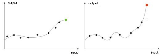
Fig. 9. Result of a "overtrained" network - wrong forecasting.

- Complexity, repeatability, inconsistency of a training sample. In works [8, 9] authors analyze dependence between the enumerated parameters. I suppose it is clear that if different teaching vectors (or, if worse, contradictory ones) correspond to one and the same learning vector, a network will never learn to classify them correctly. For this purpose large input vectors should be created, so that they contain data that allow to delimit them in the space of classes. Fig. 10 shows this dependence. The higher the complexity of a vector is, the lower is repeatability and inconsistency of patterns.

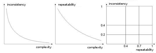
Fig. 10. Dependence of characteristics of input vectors.

- Network training by the method of Boltzmann. This method is similar to the trying of various possible weight variants. The Expert Advisor ArtificialIntelligence works according to the similar principle in its learning. When training a network, it goes through absolutely all variants of weight values (like cracking a mailbox password) and selects the best combination.

This is a labor-intensive task for a computer, that's why the number of all weights of a network is limited by ten. For example, if weight changes from 0 to 1 at the step 0.01, we will need 100 steps. For 5 weights this means 5100 combinations. This is a large number and this task is beyond the power of a computer. The only way to build a network by this method is to use a large number of computers each processing a certain part.

This task can be performed by 10 computers. Each one will process 510 combinations, so a network can be made more complex using larger number of weights, layers and steps.

As distinct from such a "Brute Force Attack", method of Boltzmann acts softer and quicker. At each iteration a random shift upon weight is set. If with the new weight the system improves its input characteristics, weight is accepted and a new iteration is made.

If a weight increases the output error, it is accepted with the probability calculated by Boltzmann distribution formula. Thus, at the beginning the network output can have absolutely different values, gradually "cooling down" bringing the network to the required global minimum [10, 11].

Of course, this is not the full list of your further studies, there are also genetic algorithms, methods for improving convergence, networks with memory, radial networks, association machines, etc.

Conclusion

I would like to add that a neuronet is not a universal cure for all your problems in trading. One selects independent work and creation of one's own algorithms, another person would prefer using ready neuro-packages, large numbers of which can be found in the market.

Just do not be afraid of experiments! Good luck to you and large profits!

Market is an intellect, financial portfolio is a neural network.

References

1. Baestaens, Dirk-Emma; Van Den Bergh, Willem Max; Wood, Douglas. Neural Network Solutions for Trading in Financial Markets.
2. Voronovskii G.K. and others. Geneticheskie algoritmy, iskusstvennye neironnye seti i problemy virtualnoy realnosti (Genetic Algoritms, Artificial Neural Networks and Problems of Virtual Reality).
3. Galushkin A.I. Teoriya Neironnyh setei (Theory of Neural Networks).
4. Debok G., Kohonen T. Analyzing Financial Data using Self-Organizing Maps.
5. Ezhov A.A., Shumckii S.A. Neirokompyuting i ego primeneniya v ekonomike i biznese (Neural Computing and Its Use in Economics and Business).
6. Ivanov D.V. Prognozirovanie finansovyh rynkov s ispolzovaniem neironnyh setei (Forcasring of Financial Maarkets Using Artificial Neural Networks) (Graduate work)
7. Osovsky S. Neural Networks for Data Processing .
8. Tarasenko R.A., Krisilov V.A., Vybor razmera opisaniya situatsii pri formirovanii obuchayushchey vyborki dlya neironnyh setei v zadachah prognozirovaniya vremennyh ryadov (Choosing the Situation Discription Size when Forming a Training Sample for Neural Networks in Tasks of Forecasting of Time Series).
9. Tarasenko R.A., Krisilov V.A., Predvaritelnaya otsenka kachestva obuchayushchey vyborki dlya neironnyh setei v zadachah prognozirovaniya vremennyh ryadov (Preliminaruy Estimation of the Quality of a training Sample for Neural Networks in Tasks of Forecasting of Time Series).
10. Philip D. Wasserman. Neral Computing: Theory and Practice.
11. Simon Haykin. Neural Networks: A Comprehensive Foundation.
12. www.wikipedia.org
13. The Internet.