MQL5 Wizard Techniques you should know (Part 10). The Unconventional RBM

Introduction

Restrictive Boltzmann Machines (RBMs) are a form of neural network that are quite simple in their structure but are none the less revered, in certain circles, for what they can accomplish when it comes to revealing hidden properties and features in data-sets. This they accomplish by learning the weights in a smaller dimension from a larger dimensioned input data, with these weights often referred to as probability distributions. As always more reading can be done here, but usually their structure can be illustrated by the image below:

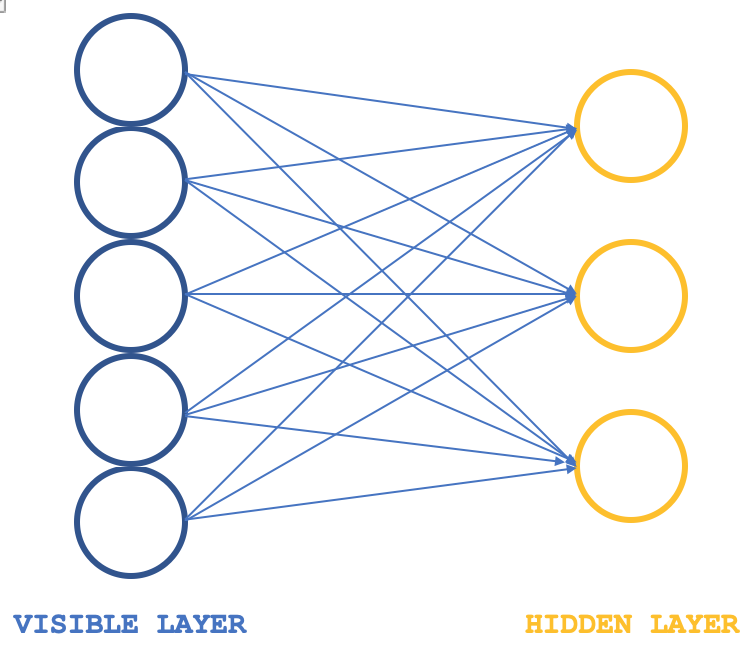
Typically, RBMs consist of 2 layers, (I say typically because there are some networks that stack them into transformers) a visible layer and a hidden layer with the visible layer being larger (having more neurons) than the hidden layer. Every neuron in the visible layer connects to each neuron in the hidden layer during what is referred to as the positive phase such that during this phase as is common with most neural networks, the input values at the visible layer gets multiplied by weight values at connecting neurons and the sum of these products gets added to a bias to determine the values at the respective hidden neurons. The negative phase which is the reverse of this is then what follows and through different neuron connections, it aims to restore the input data to its original state starting with the computed values in the hidden layer.

So, with the early cycles as one would expect the reconstructed input data is bound to mismatch the initial input because often the RBM is initialized with random weights. This implies the weights need to be adjusted to bring the reconstructed output closer to the input data and this is the additional phase that would follow each cycle. The end-result and objective of this cycle positive phase followed by a negative phase and weights adjustment, is to arrive at connecting neuron weights which when applied to input data, can give us ‘intuitive’ neuron values in the hidden layer. These neuron values in the hidden layer are what is referred to as the probability distribution of the input data across the hidden neurons.

The positive and negative phase of an RBM cycle are often collectively referred to as Gibbs Sampling. And in order to arrive at connecting weights that accurately map to the data’s probability distribution, the connecting weights are adjusted through what is called Contrastive Divergence. So, if we were to have a simple class that illustrates this in MQL5, then our interface could look as follows:

//+------------------------------------------------------------------+
//|                                                                  |
//+------------------------------------------------------------------+
class Crbm
{
protected:

... 

public:

   bool                             init;

   matrix                           weights_v_to_h;
   matrix                           weights_h_to_v;
   vector                           bias_v_to_h;
   vector                           bias_h_to_v;

   matrix                           old_visible;
   matrix                           old_hidden;
   matrix                           new_hidden;
   matrix                           new_visible;

   matrix                           output;

   void                             GibbsSample(matrix &Input);
   void                             ContrastiveDivergence();

   Crbm(int Visible, int Hidden, int Sample, double LearningRate, ENUM_LOSS_FUNCTION Loss);
   ~Crbm();
};

The notable variables here are the matrices that log the weights when propagating from the visible layer to the hidden layer and also when propagating in the reverse direction, these are aptly named ‘weights_v_to_h’ and ‘weights_h_to_v’ respectively. Also, to be included should be the vectors that log the biases and most importantly the 4 sets of neurons that are used in the Gibbs Sampling to store neuron values on each sampling; 2 for the visible layer and 2 for the hidden layer. The Gibbs Sampling for both the positive and negative phase could have its function defined as below:

//+------------------------------------------------------------------+
//| Feed through network using Gibbs Sampling                        |
//+------------------------------------------------------------------+
void Crbm::GibbsSample(matrix &Input)
{  old_visible.Fill(0.0);
   old_visible.Copy(Input);
   //old_hidden = old_visible * weights_v_to_h;
   //new_hidden = Sigmoid(old_hidden) + bias_v_to_h;
   for (int GibbsStep = 0; GibbsStep < sample; GibbsStep++)
   {  // Positive phase... Upward pass with biases
      for (int j = 0; j < hidden; j++)
      {  old_hidden[GibbsStep][j] = 0.0;
         for (int i = 0; i < visible; i++)
         {  old_hidden[GibbsStep][j] += (old_visible[GibbsStep][i] * weights_v_to_h[i][j]);
         }
         new_hidden[GibbsStep][j] = 1.0 / (1.0 + exp(-(old_hidden[GibbsStep][j] + bias_v_to_h[j])));
      }
   }
   //new_visible = new_hidden * weights_h_to_v;
   //output = Sigmoid(new_visible) + bias_v_to_h;
   for (int GibbsStep = 0; GibbsStep < sample; GibbsStep++)
   {  // Negative phase... Downward pass with biases
      for (int i = 0; i < visible; i++)
      {  new_visible[GibbsStep][i] = 0.0;
         for (int j = 0; j < hidden; j++)
         {  new_visible[GibbsStep][i] += (new_hidden[GibbsStep][j] * weights_h_to_v[j][i]);
         }
         output[GibbsStep][i] = 1.0 / (1.0 + exp(-(new_visible[GibbsStep][i] + bias_h_to_v[i])));
      }
   }
}

And similarly, the updating of the neuron weights and biases could be realized with the function below:

//+------------------------------------------------------------------+
//| Update weights using Contrastive Divergence                      |
//+------------------------------------------------------------------+
void Crbm::ContrastiveDivergence()
{  // Update weights based on the difference between positive and negative phase
   matrix _weights_v_to_h_update;
   _weights_v_to_h_update.Init(visible, hidden);
   _weights_v_to_h_update.Fill(0.0);
   matrix _weights_h_to_v_update;
   _weights_h_to_v_update.Init(hidden, visible);
   _weights_h_to_v_update.Fill(0.0);
   for (int i = 0; i < visible; i++)
   {  for (int j = 0; j < hidden; j++)
      {  _weights_v_to_h_update[i][j] = learning_rate * (
                                           (old_visible[0][i] * weights_v_to_h[i][j]) - old_hidden[0][j]
                                        );
         _weights_h_to_v_update[j][i] = learning_rate * (
                                           (new_hidden[0][j] * weights_h_to_v[j][i]) -
                                           new_visible[0][i]
                                        );
      }
   }
   // Apply weight updates
   for (int i = 0; i < visible; i++)
   {  for (int j = 0; j < hidden; j++)
      {  weights_v_to_h[i][j] += _weights_v_to_h_update[i][j];
         weights_h_to_v[j][i] += _weights_h_to_v_update[j][i];
      }
   }
   // Bias updates
   vector _bias_v_to_h_update;
   _bias_v_to_h_update.Init(hidden);
   vector _bias_h_to_v_update;
   _bias_h_to_v_update.Init(visible);
// Compute bias updates
   for (int j = 0; j < hidden; j++)
   {  _bias_v_to_h_update[j] = learning_rate * ((old_hidden[0][j] + bias_v_to_h[j]) - new_hidden[0][j]);
   }
   for (int i = 0; i < visible; i++)
   {  _bias_h_to_v_update[i] = learning_rate * ((new_visible[0][i] + bias_h_to_v[i]) - output[0][i]);
   }
// Apply bias updates
   for (int i = 0; i < visible; ++i)
   {  bias_h_to_v[i] += _bias_h_to_v_update[i];
   }
   for (int j = 0; j < hidden; ++j)
   {  bias_v_to_h[j] += _bias_v_to_h_update[j];
   }
}

With the old RBM structure even though schematically only 2 layers are shown in the illustration, the code has neuron values for 5 layers because negative & positive phase neuron values are logged after each product and also after each activation. So, the old visible layer logs the raw input data values, old hidden layer logs the first product of inputs and weights, the new hidden layer then logs the sigmoid-activated values of this product. The new visible layer logs the second product between the new hidden layer and the negative phase weights and finally the ‘output’ layer logs the activation of this product.

This orthodox approach at RBMs is presented here for exploration purposes only as it is compiled but not tested since this article is focusing on an alternate approach at designing and training RBMs. For analysis purposes though the key output of the Gibbs Sampling function would be the neuron values in the first and second ‘hidden-layers’. The double values of these two sets of neurons would capture input data properties after the network has been trained sufficiently.

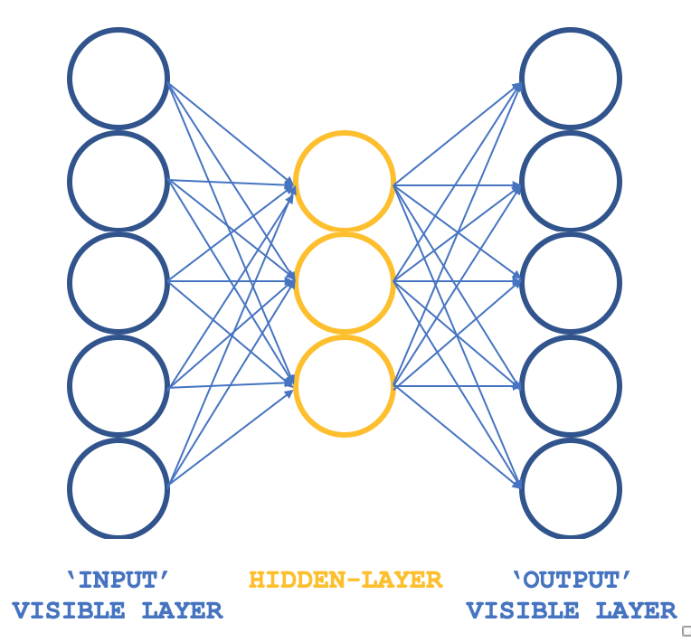
So what unconventional RBM can we look at that keeps the basic precepts but in a different structure? A 3-layer perceptron that has its input layer and output layer with matching sizes and its single hidden a size smaller than these two outer layers. How would one ensure the training is still un-supervised, since perceptrons typically have supervised learning? By having each input data row also serving as the target output, which is essentially what Gibbs Sampling is performing in each loop such that our objective of getting weights for all connections to the hidden layer can be achieved as you typically would via back propagation. The structure of our RBM would therefore resemble the image below:

This approach when used with ALGLIB classes provides a compact, and efficient approach in testing out RBMs rather than coding everything from scratch which is the theme we are exploring in these series. Once one has workable ideas then customization and perhaps coding from scratch could be considered.

Training objective to recap will be getting network weights that can accurately map features of input data in the hidden layer. These would be extracted and used in the next phase of the model and for our purposes they can be thought of as a normalized format of the input data.

RBM’s genesis

In reference to an article that was on deeplearning.net and unfortunately is no longer uploaded, RBM’s are often defined as energy-basedmodels due to their ability to associate a scalar energy to each configuration of a data set of interest. Learning is done by modifying that energy function so that its shape has desirable properties. The ‘energy function’ being a colloquial for the function involved in transforming the input data set into a different (transit) format and finally back to the input data such that the ‘energy’ is the difference between the input data set and the output data. Thus, the whole point of training RBMs is to have desirable configurations of ‘low energy’ where the difference between initial inputs and final outputs is minimized. Energy-based probabilistic models would define a probability distribution obtained via this energy function, as being the hidden neuron vector as a fraction the sum of hidden neuron values for all sampled input data.

In general energy-based models are trained by performing (stochastic) gradient descent on the empirical negative log-likelihood of the training data. And general Boltzmann machines do not have any hidden layers and all neurons are interconnected.

The first step therefore in making this computation tractable is to estimate the expectation using a fixed number of model samples. Samples used to estimate the positive phase gradient are referred to as weights, and a product of these matrix weights and the input data set vector should provide a vector of neuron values. (i.e. when doing a Monte-Carlo). With this, we'd almost have a practical, stochastic algorithm for learning an EBM. The only missing ingredient is how to extract these weights. While the statistical literature abounds with sampling methods, Markov Chain Monte Carlo methods are especially well suited for models such as the Boltzmann Machines (BM), a specific type of EBM.

Boltzmann Machines (BMs) are a particular form of log-linear Markov Random Field (MRF), i.e., for which the energy function is linear in its free parameters. To make them powerful enough to represent complicated distributions (i.e., go from the limited parametric setting to a non-parametric one), we consider that some of the variables are never observed (they are called hidden as stated above). By having more hidden variables (also called hidden units), we can increase the modeling capacity of the Boltzmann Machine (BM). Restricted Boltzmann Machines a derivative of this further restrict BMs to those without visible-visible and hidden-hidden connections as illustrated in the introductory image above.

In practice therefore, it is a given that not all aspects of a data set are readily ‘visible’, or we tend to need to introduce some non-observed variables to increase the expressive power of a model. This can be thought of as a presumption that there are aspects of the input data set that are unknown and therefore need to be investigated. This presumption therefore implies a gradient to these unknowns where gradient is the change or difference between the known data and the unknown aka 'hidden' data.

The gradient would contain two phases, which are referred to as the positive and negative phase. The terms positive and negative reflect their effect on the probability density or mapped unknowns being defined by the model. The positive phase aka first phase increases the probability of training data (by reducing the corresponding free energy), while the second phase decreases the probability of samples generated by the model to revert to the sampled data set.

So to sum up when the size of known and hidden data sets is un-defined like in un-restricted Boltzmann Machines, it is usually difficult to determine this gradient analytically, as it involves a lot of computation. That is why RBMs by predefining the number of knowns and unknowns can feasibly determine the probability distribution.

Network Architecture and Training

Our 3-layer structure illustrated above is going to be implemented using input and output layer sizes of 5 and a hidden layer size of 3. The inputs on the 5 neuron values will be current indicator values. These can be substituted by the reader as all source is attached but for this article we are using indicator value readings for Moving Average, MACD, Stochastic Oscillator, Williams Percent Range, and the Relative Vigor Index. The normalized output as mentioned above captures neuron values from the first and second hidden layer values meaning size of this output vector is double the size of our hidden layer.

All weight products and activations are handled by ALGLIB’s classes and these are customizable on a neuron by neuron basis and code was shared that shows this in a past article. For this article we are using the default values which would certainly need adjustment once this is taken a step further but for now it can serve to illustrate retrieval of data’s probability distribution.

So, the connections across this network resemble a butterfly rather than an arrow as illustrated in the diagram above

Backpropagation in a conventional neural network adjusts the connection weights by gradient descent via the multivariate chain-rule. This is not like contrastive divergence and not only is it bound to be more compute intense it could yield drastically different weights (probability distributions) from what you are supposed to get in a regular RBM. We are using it for testing runs in this article and since the full source is shared modifications to this phase can be customized.

As mentioned above backpropagation is usually supervised because you need target values to get the gradients and in our case since the input serves as the target, our modified RBM I would argue still qualifies as unsupervised.

On training, our network will have its weights adjusted such that the output is as close as possible to the input. In doing so any new data set that is fed to the network will provide key information to the neurons of the hidden layer. This information being from neurons is in an array format as one would expect. The size of this array though is double the number of neurons in the hidden layer. In the format we are adapting for testing the neurons in the hidden layer are three so this implies our output array that captures the properties from the 5 indicators we seek is sized 6.

These hidden neuron values can be taken as a normalization format of the 5 indicator values. We do not have a dimensionality reduction in this case since the properties vector is sized 6 and yet we used 5 input indicator values however if we were to use more indicators say 8 and kept the number of neurons on the hidden layer at 3, we would have a reduction.

So how do we use these values? If we stick to the view they are simply a normalization of the indicator values, they can serve as a classification vector that could be useful in comparison if we now use them in a different model where we add supervision in the form of an eventual change in price following each set of indicator values. So, all we do is compare the current values’ vector whose eventual price change is unknown to other vectors whose changes are known and a weighted average where cosine similarity between these vectors can act as the weight would provide the average forecast to the next change.

Coding the Network in MQL5

The interface to implement our strange RBM could look as indicated below:

//+------------------------------------------------------------------+
//|                                                                  |
//+------------------------------------------------------------------+
class Crbm
{
protected:

   int                              visible;
   int                              hidden;
   int                              sample;
   double                           loss;
   string                           file;

public:

   bool                             init;

... 

   CArrayDouble                     losses;

   void                             Train(matrix &W);
   void                             Process(matrix &W, matrix &XY, bool Compare = false);

   bool                             ReadWeights();
   bool                             WriteWeights();
   bool                             Writer();

   Crbm(int Visible, int Hidden, int Sample, double Loss, string File);
   ~Crbm();
};

In the interface we declare and use the basic minimum classes we would require to run a perceptron as we have in prior articles. The only notable addition is the ‘losses’ double array that helps us track the difference between the input layer and the output layer and in the process guide which networks get their exportable parameters written to file because as has been emphasized in the past, perceptrons should be tested with the ability to export tunable parameters such that when deploying or moving the expert to a production environment the learnt weights can be used readily rather than re-training from initial random weights each time.

So, the losses array simply records the cosine similarity between the input data set and the output data set for each data row on every price bar. At the end of a test run the networks’ weights or exportable parameters get written to a file if the number cosine similarities below an input threshold (the default value for this is 0.9, but it can be adjusted) is less than what was written the last time the file was logged. This threshold parameter is labelled ‘loss’.

The syntax used for multiplying weights and input values is probably more complicated than it ought to be considering ‘matrix’ and ‘vector’ are now embedded data types in MQL5. A simple multiplication of these while monitoring association and the respective row and column sizes could achieve the same result with less memory and therefore fewer compute resources.

The network function uses ALGLIB classes to initiate, train and process data sets. Customizations outside of this, with one’s own hard coded perceptron, could lead to better efficiency when testing and on deployment because ALGLIB’s code is fairly complex and ‘convoluted’ because being a library it tends to cater for a wider variety of scenarios. However, even with the out of box implementation some basic customizations such as with activation & biases can be done and their influence on the network’s performance can be very significant. This can be resourceful for an initial testing phase which is what we are exploring here.

So, with this test setup we train our unconventional RBM, on each new bar or whenever we get a new price point implying the weights we depend on to do the classification of each input data point are getting refined and adjusted with each pass. Alternative approaches at weights adjustment could be explored as well such as adjusting the weights once a quarter, or twice a year provided of course training over a decent number of years had been done prior to using the network. These are not considered here in the article but are mentioned as possible avenues the reader could pursue. The training and process functions are defined as indicated below:

//+------------------------------------------------------------------+
//|   Train Data Matrix                                              |
//+------------------------------------------------------------------+
void Crbm::Train(matrix &W)
{  for(int s = 0; s < sample; s++)
   {  for(int i = 0; i < visible; i++)
      {  xy.Set(s, i, W[s][i]);
         xy.Set(s, i + visible, W[s][i]);
      }
   }
   train.MLPTrainLM(model, xy, sample, 0.001, 2, info, report);
}

It is quite rudimentary because ALGLIB classes handle the coding. The process function is coded as follows:

//+------------------------------------------------------------------+
//|   Process New Vector                                             |
//+------------------------------------------------------------------+
void Crbm::Process(matrix &W, matrix &XY, bool Compare = false)
{  for(int w = 0; w < int(W.Rows()); w++)
   {  CRowDouble _x = CRowDouble(W.Row(w)), _y;
      base.MLPProcess(model, _x, _y);
      for(int i = 6; i < visible + 7; i++)
      {  XY[w][i - 6] = model.m_neurons[i];
      }
      //Comparison
      vector _input = _x.ToVector();
      vector _output = _y.ToVector();
      if(Compare)
      {  for(int i = 0; i < int(_input.Size()); i++)
         {  printf(__FUNCSIG__ +
                   " at: " + IntegerToString(i) +
                   " we've input: " + DoubleToString(_input[i]) +
                   " & y: " + DoubleToString(_y[i])
                  );
         }
         //Loss
         printf(__FUNCSIG__ +
                " loss is: " + DoubleToString(_output.Loss(_input, LOSS_COSINE))
               );
      }
      losses.Add(_output.Loss(_input, LOSS_COSINE));
   }
}

This function in a sense presents the algorithm’s ‘secrete sauce’ since it shows how we retrieve the hidden neuron values from the perceptron for each input data value. On each bar we retrieve these weights as a form of sampling. We output them therefore in a matrix format where input data row gives us a vector of weights.

The weights that are extracted for each input data point serve as normalized forms of the 5 indicator values and the weighted vector comparison mentioned above can be realized as follows:

//+------------------------------------------------------------------+
//| RBM Output.                                                      |
//+------------------------------------------------------------------+
double CSignalRBM::GetOutput(void)
   {
      m_close.Refresh(-1);
      
      MA.Refresh(-1);
      MACD.Refresh(-1);
      STOCH.Refresh(-1);
      WPR.Refresh(-1);
      RVI.Refresh(-1);
      
      double _output = 0.0;
      
      int _i=StartIndex();
      
      matrix _w; _w.Init(m_sample,__VISIBLE);
      
      matrix _xy; _xy.Init(m_sample,7);
      
      if(RBM.init)
      {
         for(int s=0;s<m_sample;s++)
         {
            for(int i=0;i<5;i++)
            {
               if(i==0){ _w[s][i] = MA.GetData(0,_i+s); }
               else if(i==1){ _w[s][i] = MACD.GetData(0,_i+s); }
               else if(i==2){ _w[s][i] = WPR.GetData(0,_i+s); }
               else if(i==3){ _w[s][i] = STOCH.GetData(0,_i+s); }
               else if(i==4){ _w[s][i] = RVI.GetData(0,_i+s); }
            }
            
            if(s>0){ _xy[s][2*__HIDDEN] = m_close.GetData(_i+s)-m_close.GetData(_i+s+1); }

         }
         
         RBM.Train(_w);
         RBM.Process(_w,_xy);
         
         double _w=0.0,_w_sum=0.0;
         
         vector _x0=_xy.Row(0); _x0.Resize(6);
         
         for(int s=1;s<m_sample;s++)
         {
            vector _x=_xy.Row(s); _x.Resize(6);
            double _weight=fabs(1.0+_x.Loss(_x0,LOSS_COSINE));
            
            _w+=(_weight*_xy[s][6]);
            _w_sum+=_weight;
         }
         
         if(_w_sum>0.0){ _w/=_w_sum; }
         
         _output=_w;
      }
      
      return(_output);
   }

With the last for loop we get the average likely forecast based off of the cosine similarity weighting with other data points that have a known Y (eventual price change)

We optimized this customized instance of the expert signal class on the symbol GBPUSD at the 4-hour timeframe from 2023.07.01 up to 2023.10.01 with a walk forward test from 2023.10.01 up to 2023.12.25 and obtained the following reports.

From these peeks it could be promising. Testing as usual would ideally be with the real ticks of the broker intended to trade with. And this would be ideally after appropriate changes and customizations are made not just to input data sources but probably the perceptron’s design and efficiency. The last bit is important because testing results that are reliable ought to be over extended periods of history data, so with ALGLIB source out of the box this could be challenging.

Conclusion

To sum up, we have looked at the traditional definition of an RBM network and how this could be scripted in MQL5. More importantly though we have explored how an unusual variant of this network that is structured and trained much like a simple multi-layer perceptron and examined if the ‘probability distribution’ what we referred to as output weights, could be put to use in building another custom instance of the expert signal class. The results from back and forward testing indicate there could be potential in using the system subject to more extensive testing and perhaps fine tuning of the choice of data input.

Notes

The attached code is usable once assembled with the MQL5 wizard. I have shown how this can be done in previous articles within these series however this article can also serve as a guide for those who are new to the wizard.