Data label for time series mining (Part 3)：Example for using label data

MetaTrader 5 — Expert Advisors | 13 October 2023, 14:11

3 820

Yuqiang Pan

Introduction

This article introduces how to use PyTorch Lightning and PyTorch Forecasting framework through MetaTrader5 trading platform to implement financial time series forecasting based on neural networks.

In the article, we will also explain our reasons for choosing these two frameworks and the data format we utilized.

Regarding the data, you can utilize the data produced by data labeling from my prior two articles. Since they share the same format, you can readily extend it following the methodology in this paper.

The links to the preceding two articles are:

Table of contents:

Several important Python libraries

First, let's introduce the main Python libraries we will use.

1. PyTorch Lightning

PyTorch Lightning is a deep learning framework that is specifically designed for professional AI researchers and machine learning engineers who require the utmost flexibility without compromising on scalability.

The central concept of it is to separate academic code (like model definitions, forward/backward propagation, optimizers, validation, etc.) from engineering code (like for loops, saving mechanisms, TensorBoard logs, training strategies, etc.), resulting in more streamlined and understandable code.

The primary benefits include:

High reusability- The design of it enables the code to be reused across various projects.
Easy maintenance- Thanks to its structured design, maintaining the code becomes simpler.
Clear logic- By abstracting boilerplate engineering code, machine learning code becomes easier to identify and comprehend.

Overall, PyTorch Lightning is an extremely potent library that offers an efficient method for organizing and managing your PyTorch code. Additionally, it provides a structured approach to dealing with common yet intricate tasks like model training, validation, and testing.

The detailed usage of this librarie can be found in their official documentation: https://lightning.ai/docs.

2. PyTorch Forecasting

It is a Python library that is specifically designed for time series forecasting. As it is built on PyTorch, you can leverage the powerful automatic differentiation and optimization libraries of PyTorch, while also benefiting from the convenience that PyTorch Forecasting offers for time series forecasting.

Within PyTorch Forecasting, you can find implementations of a variety of predictive models, including but not limited to autoregressive models (AR, ARIMA), state space models (SARIMAX), neural networks (LSTM, GRU), and ensemble methods (Prophet, N-Beats). This implies that you can experiment with and compare different predictive approaches within the same framework without the need to write extensive boilerplate code for each approach.

The library also offers a range of data preprocessing tools that can assist you in handling common tasks in time series. These tools encompass missing value imputation, scaling, feature extraction, and rolling window transformations among others. This implies that you can concentrate more on the design and optimization of your model without needing to devote substantial time to data processing.

It also offers a unified interface for evaluating model performance. It implements loss functions and validation metrics for time series like QuantileLoss and SMAPE, and supports training methodologies like early stopping and cross-validation. This enables you to track and enhance your model’s performance more conveniently.

If you’re seeking a method to enhance the efficiency and maintainability of your time series forecasting project, then PyTorch Forecasting might be an excellent choice. It offers an effective and flexible means to organize and manage your PyTorch code, enabling you to concentrate on the most crucial aspect - the machine learning model itself.

The detailed usage of this librarie can be found in their official documentation: https://pytorch-forecasting.readthedocs.io/en/stable.

3. About N-HiTS model

The N-HiTS model addresses the issues of prediction volatility and computational complexity in long-term forecasting by introducing innovative hierarchical interpolation and multi-rate data sampling techniques. This allows the N-HiTS model to effectively approximate a prediction range of any length.

Furthermore, extensive experiments conducted on large-scale datasets have demonstrated that the N-HiTS model improves accuracy by an average of nearly 20% compared to the latest Transformer architecture, while also reducing computation time by an order of magnitude (50 times).

Link to the paper: https://doi.org/10.48550/arXiv.2201.12886.

Initialization

First, we need to import the required libraries. These libraries include MetaTrader5 (for interacting with the MT5 terminal), PyTorch Lightning (for training the model), and some other libraries for data processing and visualization.

import MetaTrader5 as mt5
import lightning.pytorch as pl
from lightning.pytorch.callbacks import EarlyStopping
import matplotlib.pyplot as plt
import pandas as pd
from pytorch_forecasting import Baseline, NHiTS, TimeSeriesDataSet
from pytorch_forecasting.data import NaNLabelEncoder
from pytorch_forecasting.metrics import MAE, SMAPE, MQF2DistributionLoss, QuantileLoss
from lightning.pytorch.tuner import Tuner

Next, we need to initialize MetaTrader5. This is done by calling the mt.initialize() function. If you cannot initialize it simply by using it, you need to pass the path of the MT5 terminal as a parameter to this function (in the example “D:\Project\mt\MT5\terminal64.exe” is my personal path location, in actual application you need to configure it to your own path location). If initialization is successful, the function will return True, otherwise False.

if not mt.initialize("D:\\Project\\mt\\MT5\\terminal64.exe"):
    print('initialize() failed!')
else:
    print(mt.version())

The mt.symbols_total() function is used to get the total number of tradable varieties available in the MT5 terminal. We can use it to judge whether we can correctly obtain data. If the total number is greater than 0, we can use the mt.copy_rates_from_pos() function to obtain historical data of the specified tradable variety. In this example, we obtained the most recent length of "mt_data_len" M15 (15 minutes) period data of the “GOLD_micro” variety.

sb=mt.symbols_total()
rts=None
if sb > 0:
    rts=mt.copy_rates_from_pos("GOLD_micro",mt.TIMEFRAME_M15,0,mt_data_len) 
    mt.shutdown()

Finally, we use the mt.shutdown() function to close the connection with the MT5 terminal and convert the obtained data into Pandas DataFrame format.

mt.shutdown()
rts_fm=pd.DataFrame(rts)

Now, let’s discuss how to preprocess the data obtained from the MT5 terminal.

we need to convert timestamps into dates first:

rts_fm['time']=pd.to_datetime(rts_fm['time'], unit='s')

Here we no longer describe how to label data. You can find methods in my previous two articles (there are article links in the introduction of this article). For a concise demonstration of how to use prediction models, we simply divide every "max_encoder_length+2max_prediction_length" pieces of data into a group. Each group has a sequence from 0 to "max_encoder_length+2max_prediction_length-1", and fill them. In this way, we add the required labels to the original data. First we need to convert the original time index (i.e., DataFrame’s index) into a time index. Calculate the remainder of the original time index divided by (max_encoder_length+2max_prediction_length), and use the result as a new time index. This maps the time index into a range from 0 to "max_encoder_length+2*max_prediction_length-1":

rts_fm['time_idx']= rts_fm.index%(max_encoder_length+2*max_prediction_length)

We also need to convert the original time index into a group. Calculate the original time index divided by "max_encoder_length+2*max_prediction_length", and use the result as a new group:

rts_fm['series']=rts_fm.index//(max_encoder_length+2*max_prediction_length)

We encapsulate the data preprocessing part into a function. We only need to pass it the length of data we need to get and it can complete data preprocessing work:

def get_data(mt_data_len:int):
    if not mt.initialize("D:\\Project\\mt\\MT5\\terminal64.exe"):
        print('initialize() failed!') 
    else:
        print(mt.version())
        sb=mt.symbols_total()
        rts=None
        if sb > 0:
            rts=mt.copy_rates_from_pos("GOLD_micro",mt.TIMEFRAME_M15,0,mt_data_len) 
        mt.shutdown()
        # print(len(rts))
    rts_fm=pd.DataFrame(rts)
    rts_fm['time']=pd.to_datetime(rts_fm['time'], unit='s') 
    rts_fm['time_idx']= rts_fm.index%(max_encoder_length+2*max_prediction_length) 
    rts_fm['series']=rts_fm.index//(max_encoder_length+2*max_prediction_length)
return rts_fm

Rewriting the pytorch_forecasting.TimeSeriesDataSet class

Rewriting the to_dataloader() function in the pytorch_forecasting. This allows you to control whether the data is shuffled and whether to drop the last group of a batch (mainly to prevent unpredictable errors caused by insufficient length of the last group of data). Here’s how you can do it:

class New_TmSrDt(TimeSeriesDataSet):
    def to_dataloader(self, train: bool = True, 
                      batch_size: int = 64, 
                      batch_sampler: Sampler | str = None, 
                      shuffle:bool=False,
                      drop_last:bool=False,
                      **kwargs) -> DataLoader:
        default_kwargs = dict(
            shuffle=shuffle,
            drop_last=drop_last, #modification
            collate_fn=self._collate_fn,
            batch_size=batch_size,
            batch_sampler=batch_sampler,
        )
        default_kwargs.update(kwargs)
        kwargs = default_kwargs
        if kwargs["batch_sampler"] is not None:
            sampler = kwargs["batch_sampler"]
            if isinstance(sampler, str):
                if sampler == "synchronized":
                    kwargs["batch_sampler"] = TimeSynchronizedBatchSampler(
                        SequentialSampler(self),
                        batch_size=kwargs["batch_size"],
                        shuffle=kwargs["shuffle"],
                        drop_last=kwargs["drop_last"],
                    )
                else:
                    raise ValueError(f"batch_sampler {sampler} unknown - see docstring for valid batch_sampler")
            del kwargs["batch_size"]
            del kwargs["shuffle"]
            del kwargs["drop_last"]

        return DataLoader(self,**kwargs)

This code creates a new class New_TmSrDt that inherits from TimeSeriesDataSet . The to_dataloader() function is then overridden in this new class to include the shuffle and drop_last parameters. This way, you can have more control over your data loading process. Remember to replace instances of TimeSeriesDataSet with New_TmSrDt in your code.

Creating Training and Validation Datasets

First, we need to determine the cutoff point for the training data. This is done by subtracting the maximum prediction length from the maximum ‘time_idx’ value.

max_encoder_length = 2*96
max_prediction_length = 30
training_cutoff = rts_fm["time_idx"].max() - max_prediction_length

Then, we use the New_TmSrDt class (which is the TimeSeriesDataSet class we rewrote) to create a training dataset. This class requires the following parameters:

The DataFrame (in this case ‘rts_fm’)
The ‘time_idx’ column, which is a continuous integer sequence
The target column (in this case ‘close’), which is the value we want to predict
The group column (in this case ‘series’), which represents different time series
The maximum lengths of the encoder and predictor

context_length = max_encoder_length
prediction_length = max_prediction_length

training = New_TmSrDt(
        data[lambda x: x.time_idx <= training_cutoff],
        time_idx="time_idx",
        target="close",
        categorical_encoders={"series":NaNLabelEncoder().fit(data.series)},
        group_ids=["series"],
        time_varying_unknown_reals=["close"],
        max_encoder_length=context_length,
        # min_encoder_length=max_encoder_length//2,
        max_prediction_length=prediction_length,
        # min_prediction_length=1,
    )
validation = New_TmSrDt.from_dataset(training, 
                                  data, 
                                  min_prediction_idx=training_cutoff + 1)

Next, we use the New_TmSrDt.from_dataset() function to create a validation dataset. This function requires the following parameters:

The training dataset
The DataFrame
The minimum prediction index, which should be 1 greater than the maximum ‘time_idx’ value of the training data

validation = New_TmSrDt.from_dataset(training, rts_fm, min_prediction_idx=training_cutoff + 1)

Finally, we use the to_dataloader() function to convert the training and validation datasets into PyTorch DataLoader objects. This function requires the following parameters:

The ‘train’ parameter, which indicates whether the data should be shuffled
The ‘batch_size’ parameter, which specifies the number of samples per batch
The ‘num_workers’ parameter, which specifies the number of worker processes for data loading

train_dataloader = training.to_dataloader(train=True,
                                          shuffle=t_shuffle, 
                                          drop_last=t_drop_last,
                                          batch_size=batch_size, 
                                          num_workers=0,)
val_dataloader = validation.to_dataloader(train=False, 
                                          shuffle=v_shuffle,
                                          drop_last=v_drop_last,
                                          batch_size=batch_size, 
                                          num_workers=0)

Finally, we encapsulate this part of code into a function spilt_data(data:pd.DataFrame,t_drop_last:bool,t_shuffle:bool,v_drop_last:bool,v_shuffle:bool) , and specify the following parameters:

The ‘data’ parameter, which is used to receive the dataset that needs to be processed
The ‘t_drop_last’ parameter, which indicates whether the last group of the training dataset should be dropped
The ‘t_shuffle’ parameter, which indicates whether the training data should be shuffled
The ‘v_drop_last’ parameter, which indicates whether the last group of the validation dataset should be dropped
The ‘v_shuffle’ parameter, which indicates whether the validation data should be shuffled

We make train_dataloader(an instance of dataloader for training dataset), val_dataloader(an instance of dataloader for validation dataset) and training(an instance of TimeSeriesDataSet for dataset) as return values of this function as they will be used later.

def spilt_data(data:pd.DataFrame,
               t_drop_last:bool,
               t_shuffle:bool,
               v_drop_last:bool,
               v_shuffle:bool):
    training_cutoff = data["time_idx"].max() - max_prediction_length #max:95
    context_length = max_encoder_length
    prediction_length = max_prediction_length
    training = New_TmSrDt(
        data[lambda x: x.time_idx <= training_cutoff],
        time_idx="time_idx",
        target="close",
        categorical_encoders={"series":NaNLabelEncoder().fit(data.series)},
        group_ids=["series"],
        time_varying_unknown_reals=["close"],
        max_encoder_length=context_length,
        # min_encoder_length=max_encoder_length//2,
        max_prediction_length=prediction_length,
        # min_prediction_length=1,
    )

    validation = New_TmSrDt.from_dataset(training, 
                                         data, 
                                         min_prediction_idx=training_cutoff + 1)
    
    train_dataloader = training.to_dataloader(train=True,
                                              shuffle=t_shuffle, 
                                              drop_last=t_drop_last,
                                              batch_size=batch_size, 
                                              num_workers=0,)
    val_dataloader = validation.to_dataloader(train=False, 
                                              shuffle=v_shuffle,
                                              drop_last=v_drop_last,
                                              batch_size=batch_size, 
                                              num_workers=0)
    return train_dataloader,val_dataloader,training

Model Creation and Training

Now we start creating the NHiTS model. This part will show how to set its parameters and how to train it.

1.Find the best learning rate

Before starting model creation, we use the Tuner object of PyTorch Lightning to find the best learning rate.

First, we need to create a Trainer object of PyTorch Lightning, where the ‘accelerator’ parameter is used to specify the device type, and ‘gradient_clip_val’ is used to prevent gradient explosion.

pl.seed_everything(42)
trainer = pl.Trainer(accelerator="cpu", gradient_clip_val=0.1)

Next, we use the NHiTS.from_dataset() function to create an NHiTS model net . This function requires the following parameters:

The training dataset
The learning rate
Weight decay
The loss function
The size of the hidden layer
The optimizer

net = NHiTS.from_dataset(
    training,
    learning_rate=3e-2,
    weight_decay=1e-2,
    loss=MQF2DistributionLoss(prediction_length=max_prediction_length),
    backcast_loss_ratio=0.0,
    hidden_size=64,
    optimizer="AdamW",
)

Then we instantiate the Tuner class and call the lr_find() function. This function will train the model on a series of learning rates based on our dataset and compare the loss of each learning rate to get the best learning rate.

res = Tuner(trainer).lr_find(
    net, train_dataloaders=train_dataloader, val_dataloaders=val_dataloader, min_lr=1e-5, max_lr=1e-1
)
lr_=res.suggestion()

Similarly, we encapsulate this part of code that gets the best learning rate into a function get_learning_rate() , and make the obtained best learning rate as its return value:

def get_learning_rate():
    
    pl.seed_everything(42)
    trainer = pl.Trainer(accelerator="cpu", gradient_clip_val=0.1,logger=False)
    net = NHiTS.from_dataset(
        training,
        learning_rate=3e-2,
        weight_decay=1e-2,
        loss=MQF2DistributionLoss(prediction_length=max_prediction_length),
        backcast_loss_ratio=0.0,
        hidden_size=64,
        optimizer="AdamW",
    )
    res = Tuner(trainer).lr_find(
        net, train_dataloaders=t_loader, val_dataloaders=v_loader, min_lr=1e-5, max_lr=1e-1
    )
    lr_=res.suggestion()
    return lr_

If you want to visualize the learning rate, you can add the following code:

print(f"suggested learning rate: {res.suggestion()}")
fig = res.plot(show=True, suggest=True)
fig.show()

The result in this example is as follows:

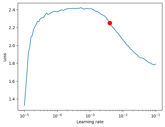
suggested learning rate: 0.003981071705534973.

2. Defining the EarlyStopping Callback

This callback is mainly used to monitor validation loss and stop training when the loss has not improved for several consecutive epochs. This can prevent model overfitting.

early_stop_callback = EarlyStopping(monitor="val_loss", 
                                    min_delta=1e-4, 
                                    patience=10,  
                                    verbose=True, 
                                    mode="min")

The parameter to note here is ‘patience’, which mainly controls when to stop during training if the loss has not improved for several consecutive epochs. We set it to 10.

3. Defining the ModelCheckpoint Callback

This callback is mainly used to control model archiving and the name of the archive. We mainly set these two variables.

ck_callback=ModelCheckpoint(monitor='val_loss',
                            mode="min",
                            save_top_k=1,  
                            filename='{epoch}-{val_loss:.2f}')

The “save_top_k” is used to control saving the top few best models. We set it to 1, only save the best model.

4. Defining the Training Model

We first need to instantiate a Trainer class in lightning.pytorch and add the two callbacks we defined earlier.

trainer = pl.Trainer(
    max_epochs=ep,
    accelerator="cpu",
    enable_model_summary=True,
    gradient_clip_val=1.0,
    callbacks=[early_stop_callback,ck_callback],
    limit_train_batches=30,
    enable_checkpointing=True,
)

The parameters we need to pay attention to here are ‘max_epochs’ (maximum number of training epochs), ‘gradient_clip_val’ (used to prevent gradient explosion), and “callbacks”. Here ‘max_epochs’ uses ep which is a global variable we will define later, and “callbacks” is our collection of callbacks.

Next, we also need to define the NHiTS model and instantiate it:

net = NHiTS.from_dataset(
    training,
    learning_rate=lr,
    log_interval=10,
    log_val_interval=1,
    weight_decay=1e-2,
    backcast_loss_ratio=0.0,
    hidden_size=64,
    optimizer="AdamW",
    loss=MQF2DistributionLoss(prediction_length=max_prediction_length),
)

Here, the parameters generally do not need to be modified, just use the default ones. Here we only modify “loss” to MQF2DistributionLoss loss function.

5. Training module

we use the fit() function of the Trainer object to train the model:

trainer.fit(
    net,
    train_dataloaders=train_dataloader,
    val_dataloaders=val_dataloader,
)

Similarly, we encapsulate this part of code into a function train() :

def train():
    early_stop_callback = EarlyStopping(monitor="val_loss", 
                                        min_delta=1e-4, 
                                        patience=10,  # The number of times without improvement will stop
                                        verbose=True, 
                                        mode="min")
    ck_callback=ModelCheckpoint(monitor='val_loss',
                                mode="min",
                                save_top_k=1,  # Save the top few best ones
                                filename='{epoch}-{val_loss:.2f}')
    trainer = pl.Trainer(
        max_epochs=ep,
        accelerator="cpu",
        enable_model_summary=True,
        gradient_clip_val=1.0,
        callbacks=[early_stop_callback,ck_callback],
        limit_train_batches=30,
        enable_checkpointing=True,
    )
    net = NHiTS.from_dataset(
        training,
        learning_rate=lr,
        log_interval=10,
        log_val_interval=1,
        weight_decay=1e-2,
        backcast_loss_ratio=0.0,
        hidden_size=64,
        optimizer="AdamW",
        loss=MQF2DistributionLoss(prediction_length=max_prediction_length),
    )
    trainer.fit(
        net,
        train_dataloaders=t_loader,
        val_dataloaders=v_loader,
        # ckpt_path='best'
    )
return trainer

This function will return a trained model that you can use for prediction tasks.

Define the execution logic

1. Defining Global Variables:

ep=200
__train=False
mt_data_len=200000
max_encoder_length = 2*96
max_prediction_length = 30
batch_size = 128

__train is used to control whether we are currently training or testing the model.

It’s worth noting that ep is used to control the maximum training epoch. Since we have set EarlyStopping, this value can be set a bit larger because the model will automatically stop when it no longer converges.

mt_data_len is the number of recent time series data obtained from the client.

max_encoder_length and max_prediction_length are respectively the maximum encoding length and maximum prediction length.

2.Training

We also need to save the current optimal training results to a local file when training is completed, so we define a json file to save this information:

info_file='results.json'

To make our training process clearer, we need to avoid outputting some unnecessary warning information during training, so we will add the following code:

warnings.filterwarnings("ignore")

Next is our training logic:

dt=get_data(mt_data_len=mt_data_len)
if __train:
    # print(dt)
    # dt=get_data(mt_data_len=mt_data_len)
    t_loader,v_loader,training=spilt_data(dt,
                                    t_shuffle=False,t_drop_last=True,
                                    v_shuffle=False,v_drop_last=True)
    lr=get_learning_rate()
    trainer__=train()
    m_c_back=trainer__.checkpoint_callback
    m_l_back=trainer__.early_stopping_callback
    best_m_p=m_c_back.best_model_path
    best_m_l=m_l_back.best_score.item()
    # print(best_m_p)
    if os.path.exists(info_file):
        with open(info_file,'r+') as f1:
            last=json.load(fp=f1)
            last_best_model=last['last_best_model']
            last_best_score=last['last_best_score']
            if last_best_score > best_m_l:
                last['last_best_model']=best_m_p
                last['last_best_score']=best_m_l
                json.dump(last,fp=f1)
    else:               
        with open(info_file,'w') as f2:
            json.dump(dict(last_best_model=best_m_p,last_best_score=best_m_l),fp=f2)

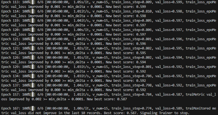
When training is completed, you can find the storage location of our best model and the best score in the results.json file in the root directory.

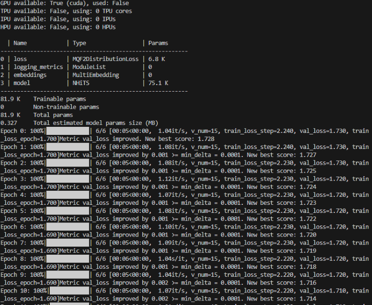
During the training process, you will see a progress bar that shows the progress of each epoch.

Training：

training

Training complete：

3. Validating the Model

After training, we want to validate the model and visualize it. We can add the following code:

best_model = NHiTS.load_from_checkpoint(best_m_p)
predictions = best_model.predict(v_loader, trainer_kwargs=dict(accelerator="cpu",logger=False), return_y=True)
raw_predictions = best_model.predict(v_loader, mode="raw", return_x=True, trainer_kwargs=dict(accelerator="cpu",logger=False))
for idx in range(10):  # plot 10 examples
    best_model.plot_prediction(raw_predictions.x, raw_predictions.output, idx=idx, add_loss_to_title=True)
    # sample 500 paths
samples = best_model.loss.sample(raw_predictions.output["prediction"][[0]], n_samples=500)[0]

# plot prediction
fig = best_model.plot_prediction(raw_predictions.x, raw_predictions.output, idx=0, add_loss_to_title=True)
ax = fig.get_axes()[0]
# plot first two sampled paths
ax.plot(samples[:, 0], color="g", label="Sample 1")
ax.plot(samples[:, 1], color="r", label="Sample 2")
fig.legend()
plt.show()

You can also use TensorBoard to view the visualization of the training situation in real time during training, we are not doing a demonstration here.

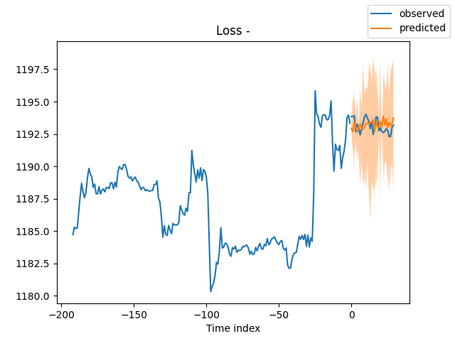
Result：

ref

4. Testing the Trained Model

First, we open the json file to find the optimal model storage location:

with open(info_file) as f:
    best_m_p=json.load(fp=f)['last_best_model']
print('model path is:',best_m_p)

Then load the model:

best_model = NHiTS.load_from_checkpoint(best_m_p)

Then we get data from the client in real time for testing the model:

offset=1
dt=dt.iloc[-max_encoder_length-offset:-offset,:]
last_=dt.iloc[-1] #get the last group of data
# print(len(dt))
for i in range(1,max_prediction_length+1):
    dt.loc[dt.index[-1]+1]=last_
dt['series']=0
# dt['time_idx']=dt.apply(lambda x:x.index,args=1)
dt['time_idx']=dt.index-dt.index[0]
# dt=get_data(mt_data_len=max_encoder_length)
predictions=best_model.predict(dt,mode='raw',trainer_kwargs=dict(accelerator="cpu",logger=False),return_x=True)
best_model.plot_prediction(predictions.x,predictions.output,show_future_observed=False)
plt.show()

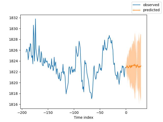
The result is as follows:

pref

5. Evaluate the model

Of course, we can use some metrics in the PyTorch Forecasting library to evaluate the performance of the model. Here is how to evaluate using Mean Absolute Error (MAE) and Symmetric Mean Absolute Percentage Error (SMAPE), and output the evaluation results:

from pytorch_forecasting.metrics import MAE, SMAPE
mae = MAE()(raw_predictions["prediction"], raw_predictions["target"])
print(f"Mean Absolute Error: {mae}")
smape = SMAPE()(raw_predictions["prediction"], raw_predictions["target"])
print(f"Symmetric Mean Absolute Percentage Error: {smape}")

In this code snippet, we first import the MAE and SMAPE metrics. Then we use these metrics to calculate the error between the predicted values ( raw_predictions["prediction"] ) and actual values ( raw_predictions["target"] ). These metrics can help us understand the performance of our model and provide direction for further improvement of our model.

Conclusion

In this article we looked at how to use the label data we mentioned in our previous two articles and demonstrate how to create an N-HiTs model using our data. Then we trained the model and verified the model. And we can easily see from the result chart that our results are good. We also demonstrated how to use this model in MT5 to make predictions of 30 candlesticks. Of course, we did not mention how to place orders based on the prediction results, because real trading requires readers to do a lot of testing according to your actual situation and specify the corresponding trading rules.

The end, have a good time!

Attach:

The Complete code:

# Copyright 2021, MetaQuotes Ltd.
# https://www.mql5.com


# from typing import Union
import lightning.pytorch as pl
import os
from lightning.pytorch.callbacks import EarlyStopping,ModelCheckpoint
import matplotlib.pyplot as plt
import numpy as np
import pandas as pd
# import torch
from pytorch_forecasting import NHiTS, TimeSeriesDataSet
from pytorch_forecasting.data import NaNLabelEncoder,timeseries
from pytorch_forecasting.metrics import MQF2DistributionLoss
from pytorch_forecasting.data.samplers import TimeSynchronizedBatchSampler
from lightning.pytorch.tuner import Tuner
import MetaTrader5 as mt
import warnings
import json


from torch.utils.data import DataLoader
from torch.utils.data.sampler import Sampler,SequentialSampler

class New_TmSrDt(TimeSeriesDataSet):
    '''
    rewrite dataset class
    '''
    def to_dataloader(self, train: bool = True, 
                      batch_size: int = 64, 
                      batch_sampler: Sampler | str = None, 
                      shuffle:bool=False,
                      drop_last:bool=False,
                      **kwargs) -> DataLoader:

        default_kwargs = dict(
            shuffle=shuffle,
            # drop_last=train and len(self) > batch_size,
            drop_last=drop_last, #
            collate_fn=self._collate_fn,
            batch_size=batch_size,
            batch_sampler=batch_sampler,
        )
        default_kwargs.update(kwargs)
        kwargs = default_kwargs
        # print(kwargs['drop_last'])
        if kwargs["batch_sampler"] is not None:
            sampler = kwargs["batch_sampler"]
            if isinstance(sampler, str):
                if sampler == "synchronized":
                    kwargs["batch_sampler"] = TimeSynchronizedBatchSampler(
                        SequentialSampler(self),
                        batch_size=kwargs["batch_size"],
                        shuffle=kwargs["shuffle"],
                        drop_last=kwargs["drop_last"],
                    )
                else:
                    raise ValueError(f"batch_sampler {sampler} unknown - see docstring for valid batch_sampler")
            del kwargs["batch_size"]
            del kwargs["shuffle"]
            del kwargs["drop_last"]

        return DataLoader(self,**kwargs)

def get_data(mt_data_len:int):
    if not mt.initialize():
        print('initialize() failed!') 
    else:
        print(mt.version())
        sb=mt.symbols_total()
        rts=None
        if sb > 0:
            rts=mt.copy_rates_from_pos("GOLD_micro",mt.TIMEFRAME_M15,0,mt_data_len) 
        mt.shutdown()
        # print(len(rts))
    rts_fm=pd.DataFrame(rts)
    rts_fm['time']=pd.to_datetime(rts_fm['time'], unit='s') 

    rts_fm['time_idx']= rts_fm.index%(max_encoder_length+2*max_prediction_length) 
    rts_fm['series']=rts_fm.index//(max_encoder_length+2*max_prediction_length)
    return rts_fm


def spilt_data(data:pd.DataFrame,
               t_drop_last:bool,
               t_shuffle:bool,
               v_drop_last:bool,
               v_shuffle:bool):
    training_cutoff = data["time_idx"].max() - max_prediction_length #max:95
    context_length = max_encoder_length
    prediction_length = max_prediction_length
    training = New_TmSrDt(
        data[lambda x: x.time_idx <= training_cutoff],
        time_idx="time_idx",
        target="close",
        categorical_encoders={"series":NaNLabelEncoder().fit(data.series)},
        group_ids=["series"],
        time_varying_unknown_reals=["close"],
        max_encoder_length=context_length,
        # min_encoder_length=max_encoder_length//2,
        max_prediction_length=prediction_length,
        # min_prediction_length=1,
    )

    validation = New_TmSrDt.from_dataset(training, 
                                         data, 
                                         min_prediction_idx=training_cutoff + 1)
    
    train_dataloader = training.to_dataloader(train=True,
                                              shuffle=t_shuffle, 
                                              drop_last=t_drop_last,
                                              batch_size=batch_size, 
                                              num_workers=0,)
    val_dataloader = validation.to_dataloader(train=False, 
                                              shuffle=v_shuffle,
                                              drop_last=v_drop_last,
                                              batch_size=batch_size, 
                                              num_workers=0)
    return train_dataloader,val_dataloader,training

def get_learning_rate():
    
    pl.seed_everything(42)
    trainer = pl.Trainer(accelerator="cpu", gradient_clip_val=0.1,logger=False)
    net = NHiTS.from_dataset(
        training,
        learning_rate=3e-2,
        weight_decay=1e-2,
        loss=MQF2DistributionLoss(prediction_length=max_prediction_length),
        backcast_loss_ratio=0.0,
        hidden_size=64,
        optimizer="AdamW",
    )
    res = Tuner(trainer).lr_find(
        net, train_dataloaders=t_loader, val_dataloaders=v_loader, min_lr=1e-5, max_lr=1e-1
    )
    # print(f"suggested learning rate: {res.suggestion()}")
    lr_=res.suggestion()
    return lr_
def train():
    early_stop_callback = EarlyStopping(monitor="val_loss", 
                                        min_delta=1e-4, 
                                        patience=10,  
                                        verbose=True, 
                                        mode="min")
    ck_callback=ModelCheckpoint(monitor='val_loss',
                                mode="min",
                                save_top_k=1,  
                                filename='{epoch}-{val_loss:.2f}')
    trainer = pl.Trainer(
        max_epochs=ep,
        accelerator="cpu",
        enable_model_summary=True,
        gradient_clip_val=1.0,
        callbacks=[early_stop_callback,ck_callback],
        limit_train_batches=30,
        enable_checkpointing=True,
    )
    net = NHiTS.from_dataset(
        training,
        learning_rate=lr,
        log_interval=10,
        log_val_interval=1,
        weight_decay=1e-2,
        backcast_loss_ratio=0.0,
        hidden_size=64,
        optimizer="AdamW",
        loss=MQF2DistributionLoss(prediction_length=max_prediction_length),
    )
    trainer.fit(
        net,
        train_dataloaders=t_loader,
        val_dataloaders=v_loader,
        # ckpt_path='best'
    )
    return trainer

if __name__=='__main__':
    ep=200
    __train=False
    mt_data_len=200000
    max_encoder_length = 2*96
    max_prediction_length = 30
    batch_size = 128
    info_file='results.json'
    warnings.filterwarnings("ignore")
    dt=get_data(mt_data_len=mt_data_len)
    if __train:
        # print(dt)
        # dt=get_data(mt_data_len=mt_data_len)
        t_loader,v_loader,training=spilt_data(dt,
                                              t_shuffle=False,t_drop_last=True,
                                              v_shuffle=False,v_drop_last=True)
        lr=get_learning_rate()
        trainer__=train()
        m_c_back=trainer__.checkpoint_callback
        m_l_back=trainer__.early_stopping_callback
        best_m_p=m_c_back.best_model_path
        best_m_l=m_l_back.best_score.item()

        # print(best_m_p)
        
        if os.path.exists(info_file):
            with open(info_file,'r+') as f1:
                last=json.load(fp=f1)
                last_best_model=last['last_best_model']
                last_best_score=last['last_best_score']
                if last_best_score > best_m_l:
                    last['last_best_model']=best_m_p
                    last['last_best_score']=best_m_l
                    json.dump(last,fp=f1)
        else:               
            with open(info_file,'w') as f2:
                json.dump(dict(last_best_model=best_m_p,last_best_score=best_m_l),fp=f2)

        best_model = NHiTS.load_from_checkpoint(best_m_p)
        predictions = best_model.predict(v_loader, trainer_kwargs=dict(accelerator="cpu",logger=False), return_y=True)
        raw_predictions = best_model.predict(v_loader, mode="raw", return_x=True, trainer_kwargs=dict(accelerator="cpu",logger=False))
    
        for idx in range(10):  # plot 10 examples
            best_model.plot_prediction(raw_predictions.x, raw_predictions.output, idx=idx, add_loss_to_title=True)
        samples = best_model.loss.sample(raw_predictions.output["prediction"][[0]], n_samples=500)[0]

        # plot prediction
        fig = best_model.plot_prediction(raw_predictions.x, raw_predictions.output, idx=0, add_loss_to_title=True)
        ax = fig.get_axes()[0]
        # plot first two sampled paths
        ax.plot(samples[:, 0], color="g", label="Sample 1")
        ax.plot(samples[:, 1], color="r", label="Sample 2")
        fig.legend()
        plt.show()
    else:
        with open(info_file) as f:
            best_m_p=json.load(fp=f)['last_best_model']
        print('model path is:',best_m_p)
        
        best_model = NHiTS.load_from_checkpoint(best_m_p)

        offset=1
        dt=dt.iloc[-max_encoder_length-offset:-offset,:]
        last_=dt.iloc[-1] 
        # print(len(dt))
        for i in range(1,max_prediction_length+1):
            dt.loc[dt.index[-1]+1]=last_
        dt['series']=0
        # dt['time_idx']=dt.apply(lambda x:x.index,args=1)
        dt['time_idx']=dt.index-dt.index[0]
        # dt=get_data(mt_data_len=max_encoder_length)
        predictions = best_model.predict(dt, mode='raw',trainer_kwargs=dict(accelerator="cpu",logger=False),return_x=True)
        best_model.plot_prediction(predictions.x,predictions.output,show_future_observed=False)
        plt.show()

Attached files |

Download ZIP

n_hits.py (9.7 KB)

Warning: All rights to these materials are reserved by MetaQuotes Ltd. Copying or reprinting of these materials in whole or in part is prohibited.