
Gradient Boosting (CatBoost) in the development of trading systems. A naive approach
Introduction
Gradient boosting is a powerful machine learning algorithm. The method produces an ensemble of weak models (for example, decision trees), in which (in contrast to bagging) models are built sequentially, rather than independently (in parallel). This means that the next tree learns from the mistakes of the previous one, then this process is repeated, increasing the number of weak models. This builds a strong model which can generalize using heterogeneous data. In this experiment, I used the CatBoost library developed by Yandex. It is one of the most popular libraries, along with XGboost and LightGBM.
The purpose of the article is to demonstrate the creation of a model based on machine learning. The creation process consists of the following steps:
- receive and preprocess data
- train the model using the prepared data
- test the model in a custom strategy tester
- port the model to MetaTrader 5
The Python language and the MetaTrader 5 library are used for preparing the data and for training the model.
Preparing Data
Import the required Python modules:
import MetaTrader5 as mt5
import pandas as pd
import numpy as np
from datetime import datetime
import random
import matplotlib.pyplot as plt
from catboost import CatBoostClassifier
from sklearn.model_selection import train_test_split

mt5.initialize()

# check for gpu devices is availible
from catboost.utils import get_gpu_device_count
print('%i GPU devices' % get_gpu_device_count())
Then initialize all global variables:
LOOK_BACK = 250
MA_PERIOD = 15
SYMBOL = 'EURUSD'
MARKUP = 0.0001
TIMEFRAME = mt5.TIMEFRAME_H1
START = datetime(2020, 5, 1)
STOP = datetime(2021, 1, 1)
These parameters are responsible for the following:
- look_back — depth of the analyzed history
- ma_period — moving average period for calculating price increments
- symbol — which symbol quotes should be loaded from the MetaTrader 5 terminal
- markup — spread size for a custom tester
- timeframe — timeframe data for which will be loaded
- start, stop — data range
Let us write a function that directly receives raw data and creates a dataframe containing the columns necessary for training:
def get_prices(look_back = 15):
    prices = pd.DataFrame(mt5.copy_rates_range(SYMBOL, TIMEFRAME, START, STOP),
                            columns=['time', 'close']).set_index('time')
    # set df index as datetime
    prices.index = pd.to_datetime(prices.index, unit='s')
    prices = prices.dropna()
    ratesM = prices.rolling(MA_PERIOD).mean()
    ratesD = prices - ratesM
    for i in range(look_back):
        prices[str(i)] = ratesD.shift(i)
    return prices.dropna()
The function receives close prices for the specified timeframe and calculates the moving average, after which it calculates the increments (the difference between prices and the moving average). In the final step, it calculates additional columns with rows shifted backward into history by look_back, which means adding extra (lagging) features to the model.
For example, for look_back = 10, the dataframe will contain 10 additional columns with price increments:
>>> pr = get_prices(look_back=LOOK_BACK)
>>> pr
                       close         0         1         2         3         4         5         6         7         8         9
time
2020-05-01 16:00:00  1.09750  0.001405  0.002169  0.001600  0.002595  0.002794  0.002442  0.001477  0.001190  0.000566  0.000285
2020-05-01 17:00:00  1.10074  0.004227  0.001405  0.002169  0.001600  0.002595  0.002794  0.002442  0.001477  0.001190  0.000566
2020-05-01 18:00:00  1.09976  0.002900  0.004227  0.001405  0.002169  0.001600  0.002595  0.002794  0.002442  0.001477  0.001190
2020-05-01 19:00:00  1.09874  0.001577  0.002900  0.004227  0.001405  0.002169  0.001600  0.002595  0.002794  0.002442  0.001477
2020-05-01 20:00:00  1.09817  0.000759  0.001577  0.002900  0.004227  0.001405  0.002169  0.001600  0.002595  0.002794  0.002442
...                      ...       ...       ...       ...       ...       ...       ...       ...       ...       ...       ...
2020-11-02 23:00:00  1.16404  0.000400  0.000105 -0.000581 -0.001212 -0.000999 -0.000547 -0.000344 -0.000773 -0.000326  0.000501
2020-11-03 00:00:00  1.16392  0.000217  0.000400  0.000105 -0.000581 -0.001212 -0.000999 -0.000547 -0.000344 -0.000773 -0.000326
2020-11-03 01:00:00  1.16402  0.000270  0.000217  0.000400  0.000105 -0.000581 -0.001212 -0.000999 -0.000547 -0.000344 -0.000773
2020-11-03 02:00:00  1.16423  0.000465  0.000270  0.000217  0.000400  0.000105 -0.000581 -0.001212 -0.000999 -0.000547 -0.000344
2020-11-03 03:00:00  1.16464  0.000885  0.000465  0.000270  0.000217  0.000400  0.000105 -0.000581 -0.001212 -0.000999 -0.000547

[3155 rows x 11 columns]
The yellow highlighting indicates that each column has the same dataset, but with an offset. Thus, each row is a separate training example.
Creating Training Labels (Random Sampling)
The training examples are collections of features and their corresponding labels. The model must output certain information, which the model must learn to predict. Let us consider binary classification, in which the model will predict the probability of determining the training example as class 0 or 1. Zeros and ones can be used for trade direction: buy or sell. In other words, the model must learn to predict the direction of a trade for the given environment parameters (set of features).
def add_labels(dataset, min, max):
    labels = []
    for i in range(dataset.shape[0]-max):
        rand = random.randint(min, max)
        if dataset['close'][i] >= (dataset['close'][i + rand]):
            labels.append(1.0)
        elif dataset['close'][i] <= (dataset['close'][i + rand]):
            labels.append(0.0)
        else:
            labels.append(0.0)
    dataset = dataset.iloc[:len(labels)].copy()
    dataset['labels'] = labels
    dataset = dataset.dropna()
    return dataset
The add_labels function randomly (in the min, max range) sets the duration of each deal in bars. By changing the maximum and minimum duration, you change the deal sampling frequency. Thus, if the current price is greater than the next one 'rand' bars forward, this is a sell label (1). In the opposite case, the label is 0. Let us see how the dataset looks after applying the above function:
>>> pr = add_labels(pr, 10, 25)
>>> pr
                       close         0         1         2         3         4         5         6         7         8         9  labels
time
2020-05-01 16:00:00  1.09750  0.001405  0.002169  0.001600  0.002595  0.002794  0.002442  0.001477  0.001190  0.000566  0.000285     1.0
2020-05-01 17:00:00  1.10074  0.004227  0.001405  0.002169  0.001600  0.002595  0.002794  0.002442  0.001477  0.001190  0.000566     1.0
2020-05-01 18:00:00  1.09976  0.002900  0.004227  0.001405  0.002169  0.001600  0.002595  0.002794  0.002442  0.001477  0.001190     1.0
2020-05-01 19:00:00  1.09874  0.001577  0.002900  0.004227  0.001405  0.002169  0.001600  0.002595  0.002794  0.002442  0.001477     1.0
2020-05-01 20:00:00  1.09817  0.000759  0.001577  0.002900  0.004227  0.001405  0.002169  0.001600  0.002595  0.002794  0.002442     1.0
...                      ...       ...       ...       ...       ...       ...       ...       ...       ...       ...       ...     ...
2020-10-29 20:00:00  1.16700 -0.003651 -0.005429 -0.005767 -0.006750 -0.004699 -0.004328 -0.003475 -0.003769 -0.002719 -0.002075     1.0
2020-10-29 21:00:00  1.16743 -0.002699 -0.003651 -0.005429 -0.005767 -0.006750 -0.004699 -0.004328 -0.003475 -0.003769 -0.002719     0.0
2020-10-29 22:00:00  1.16731 -0.002276 -0.002699 -0.003651 -0.005429 -0.005767 -0.006750 -0.004699 -0.004328 -0.003475 -0.003769     0.0
2020-10-29 23:00:00  1.16740 -0.001648 -0.002276 -0.002699 -0.003651 -0.005429 -0.005767 -0.006750 -0.004699 -0.004328 -0.003475     0.0
2020-10-30 00:00:00  1.16695 -0.001655 -0.001648 -0.002276 -0.002699 -0.003651 -0.005429 -0.005767 -0.006750 -0.004699 -0.004328     1.0
The 'labels' column has been added, which contains the class number (0 or 1) for buy and sell, respectively. Now, each training example or set of features (which are 10 here) has its own label, which indicates under which conditions you should buy, and under which conditions you should sell (i.e. to which class it belongs). The model must be able to remember and generalize these examples — this ability will be discussed later.
Developing a Custom Tester
Since we are creating a trading system, it would be nice to have a Strategy Tester for timely model testing. Below is an example of such a tester:
def tester(dataset, markup = 0.0):
    last_deal = int(2)
    last_price = 0.0
    report = [0.0]
    for i in range(dataset.shape[0]):
        pred = dataset['labels'][i]
        if last_deal == 2:
            last_price = dataset['close'][i]
            last_deal = 0 if pred <=0.5 else 1
            continue
        if last_deal == 0 and pred > 0.5:
            last_deal = 1
            report.append(report[-1] - markup + (dataset['close'][i] - last_price))
            last_price = dataset['close'][i]
            continue
        if last_deal == 1 and pred <=0.5:
            last_deal = 0
            report.append(report[-1] - markup + (last_price - dataset['close'][i]))
            last_price = dataset['close'][i]
    return report
The tester function accepts a dataset and a 'markup' (optional) and checks the entire dataset, similarly to how it is done in the MetaTrader 5 tester. A signal (label) is checked at each new bar and when the label changes, the trade is reversed. Thus, a sell signal serves as a signal to close a buy position and to open a sell position. Now, let us test the above dataset:
pr = get_prices(look_back=LOOK_BACK)
pr = add_labels(pr, 10, 25)
rep = tester(pr, MARKUP)
plt.plot(rep)
plt.show()
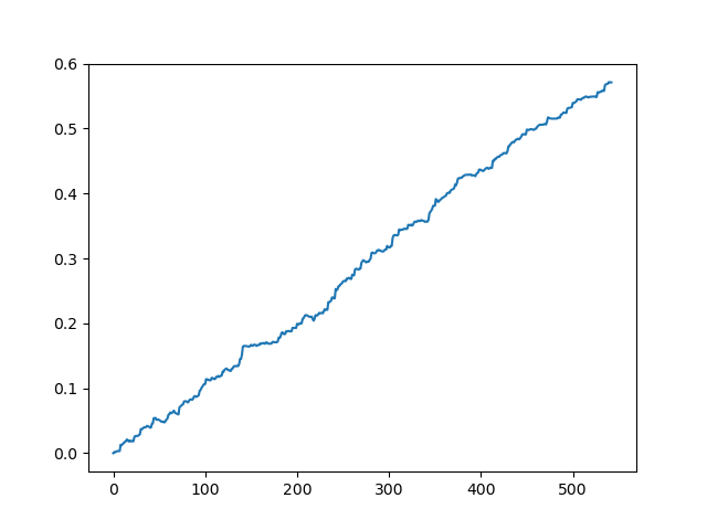
Testing the original dataset without spread
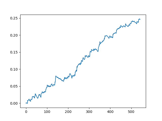
Testing the original dataset with a spread of 70 five-digit points
This is a kind of idealized picture (this is how we want the model to work). Since labels are sampled randomly, depending on a range of parameters responsible for the minimum and maximum lifetime of trades, the curves will always be different. Nevertheless, they will all show a good point increase (along the Y axis) and a different number of trades (along the X axis).
Training the CatBoost Model
Now, let us move on directly to training the model. First, let us split the dataset into two samples: training and validation. This is used to reduce model overfitting. While the model continues to train on the training subsample, trying to minimize the classification error, the same error is also measured on the validation subsample. If the difference in these errors is great, the model is said to be overfit. Conversely, close values indicate proper training of a model.
#splitting on train and validation subsets
X = pr[pr.columns[1:-1]]
y = pr[pr.columns[-1]]
train_X, test_X, train_y, test_y = train_test_split(X, y, train_size = 0.5, test_size = 0.5, shuffle=True)
Let us split the data into two datasets having equal lengths, after randomly mixing the training examples. Next, create and train the model:
#learning with train and validation subsets
model = CatBoostClassifier(iterations=1000,
                        depth=6,
                        learning_rate=0.01,
                        custom_loss=['Accuracy'],
                        eval_metric='Accuracy',
                        verbose=True,
                        use_best_model=True,
                        task_type='CPU')
model.fit(train_X, train_y, eval_set = (test_X, test_y), early_stopping_rounds=50, plot=False)
The model takes a number of parameters, while not all of them are shown in this example. You can refer to the documentation, if you wish to fine-tune the model, which is not required as a rule. CatBoost works well out of the box, with minimal tuning.
Here is a brief description of model parameters:
- iterations — the maximum number of trees in the model. The model increases the number of weak models (trees) after each iteration, so make sure to set a large enough value. From my practice, 1000 iterations for this particular example are normally more than enough.
- depth — the depth of each tree. The smaller the depth, the coarser the model - outputting less trades. The depth between 6 and 10 seems optimal.
- learning_rate — gradient step value; this is the same principle used in neural networks. A reasonable range of parameters is 0.01 - 0.1. The lower the value, the longer the model takes to train. But in this case it can find better variants.
- custom_loss, eval_metric — the metric used to evaluate the model. The classical metric for classification is 'accuracy'
- use_best_model — at each step, the model evaluates 'accuracy', which can change over time. This flag allows saving the model with the least error. Otherwise the model obtained at the last iteration will be saved
- task_type — allows training a model on a GPU (CPU is used by default). This is only relevant in the case of very large data; in other cases training is performed more slowly on GPU cores than on the processor.
- early_stopping_rounds — the model has a built-in overfitting detector which operates according to a simple principle. If the metric stops decreasing/increasing (for 'accuracy' it stops increasing) during the specified number of iterations, then training stops.
After training starts, the current state of the model at each iteration will be displayed in the console:
170:    learn: 1.0000000        test: 0.7712509 best: 0.7767795 (165)   total: 11.2s    remaining: 21.5s
171:    learn: 1.0000000        test: 0.7726330 best: 0.7767795 (165)   total: 11.2s    remaining: 21.4s
172:    learn: 1.0000000        test: 0.7733241 best: 0.7767795 (165)   total: 11.3s    remaining: 21.3s
173:    learn: 1.0000000        test: 0.7740152 best: 0.7767795 (165)   total: 11.3s    remaining: 21.3s
174:    learn: 1.0000000        test: 0.7712509 best: 0.7767795 (165)   total: 11.4s    remaining: 21.2s
175:    learn: 1.0000000        test: 0.7726330 best: 0.7767795 (165)   total: 11.5s    remaining: 21.1s
176:    learn: 1.0000000        test: 0.7712509 best: 0.7767795 (165)   total: 11.5s    remaining: 21s
177:    learn: 1.0000000        test: 0.7740152 best: 0.7767795 (165)   total: 11.6s    remaining: 21s
178:    learn: 1.0000000        test: 0.7719419 best: 0.7767795 (165)   total: 11.7s    remaining: 20.9s
179:    learn: 1.0000000        test: 0.7747063 best: 0.7767795 (165)   total: 11.7s    remaining: 20.8s
180:    learn: 1.0000000        test: 0.7705598 best: 0.7767795 (165)   total: 11.8s    remaining: 20.7s
Stopped by overfitting detector  (15 iterations wait)

bestTest = 0.7767795439
bestIteration = 165
In the above example, overfitting detector triggered and stopped training at iteration 180. Also, the console displays statistics for the training subsample (learn) and validation subsample (test), as well as the total model training time, which was only 20 seconds. At the output, we got the best accuracy on the training subsample 1.0 (which corresponds to the ideal result) and the accuracy of 0.78 on the validation subsample, which is worse but is still above 0.5 (which is considered random). The best iteration is 165 — this model is saved. Now, we can test in our Tester:
#test the learned model
p = model.predict_proba(X)
p2 = [x[0]<0.5 for x in p]
pr2 = pr.iloc[:len(p2)].copy()
pr2['labels'] = p2
rep = tester(pr2, MARKUP)
plt.plot(rep)
plt.show()
X - is the source dataset with features but without labels. To get the labels, it is necessary to obtain them from the trained model and to predict the 'p' probabilities of assignment to class 0 or 1. Since the model generates the probabilities for two classes, while we need only 0s or 1s, the 'p2' variable receives probabilities only in the first dimension (0). Further, the labels in the original dataset are replaced with the labels predicted by the model. Here are the results in the Tester:
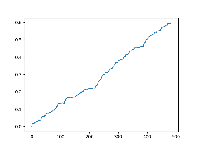
An ideal result after sampling trades
The result obtained at the model output
As you can see, the model has learned well, which means it remembered the training examples and has shown a better than random result on the validation set. Let us move on to the final stage: exporting the model and creating a trading robot.
Porting the Model to MetaTrader 5
MetaTrader 5 Python API allows trading directly from a python program and thus there is no need to port the model. However, I wanted to check my custom tester and compare it with the standard Strategy Tester. Furthermore, the availability of a compiled bot can be convenient in many situations, including the usage on a VPS (in this case you will not have to install Python). So, I have written a helper function that saves a ready model to an MQH file. The function is as follows:
def export_model_to_MQL_code(model):
    model.save_model('catmodel.h',
           format="cpp",
           export_parameters=None,
           pool=None)
    code = 'double catboost_model' + '(const double &features[]) { \n'
    code += '    '
    with open('catmodel.h', 'r') as file:
        data = file.read()
        code += data[data.find("unsigned int TreeDepth"):data.find("double Scale = 1;")]
    code +='\n\n'
    code+= 'return ' + 'ApplyCatboostModel(features, TreeDepth, TreeSplits , BorderCounts, Borders, LeafValues); } \n\n'

    code += 'double ApplyCatboostModel(const double &features[],uint &TreeDepth_[],uint &TreeSplits_[],uint &BorderCounts_[],float &Borders_[],double &LeafValues_[]) {\n\
    uint FloatFeatureCount=ArrayRange(BorderCounts_,0);\n\
    uint BinaryFeatureCount=ArrayRange(Borders_,0);\n\
    uint TreeCount=ArrayRange(TreeDepth_,0);\n\
    bool     binaryFeatures[];\n\
    ArrayResize(binaryFeatures,BinaryFeatureCount);\n\
    uint binFeatureIndex=0;\n\
    for(uint i=0; i<FloatFeatureCount; i++) {\n\
       for(uint j=0; j<BorderCounts_[i]; j++) {\n\
          binaryFeatures[binFeatureIndex]=features[i]>Borders_[binFeatureIndex];\n\
          binFeatureIndex++;\n\
       }\n\
    }\n\
    double result=0.0;\n\
    uint treeSplitsPtr=0;\n\
    uint leafValuesForCurrentTreePtr=0;\n\
    for(uint treeId=0; treeId<TreeCount; treeId++) {\n\
       uint currentTreeDepth=TreeDepth_[treeId];\n\
       uint index=0;\n\
       for(uint depth=0; depth<currentTreeDepth; depth++) {\n\
          index|=(binaryFeatures[TreeSplits_[treeSplitsPtr+depth]]<<depth);\n\
       }\n\
       result+=LeafValues_[leafValuesForCurrentTreePtr+index];\n\
       treeSplitsPtr+=currentTreeDepth;\n\
       leafValuesForCurrentTreePtr+=(1<<currentTreeDepth);\n\
    }\n\
    return 1.0/(1.0+MathPow(M_E,-result));\n\
    }'

    file = open('C:/Users/dmitrievsky/AppData/Roaming/MetaQuotes/Terminal/D0E8209F77C8CF37AD8BF550E51FF075/MQL5/Include/' + 'cat_model' + '.mqh', "w")
    file.write(code)
    file.close()
    print('The file ' + 'cat_model' + '.mqh ' + 'has been written to disc')
The function code looks strange and awkward. The trained model object is input into the function, which then saves the object in a C++ format:
model.save_model('catmodel.h',
           format="cpp",
           export_parameters=None,
           pool=None)
Then a string is created, and the C++ code is parsed into MQL5 using standard Python functions:
code = 'double catboost_model' + '(const double &features[]) { \n'
    code += '    '
    with open('catmodel.h', 'r') as file:
        data = file.read()
        code += data[data.find("unsigned int TreeDepth"):data.find("double Scale = 1;")]
    code +='\n\n'
    code+= 'return ' + 'ApplyCatboostModel(features, TreeDepth, TreeSplits , BorderCounts, Borders, LeafValues); } \n\n'
The 'ApplyCatboostModel' function from this library is inserted after the above manipulations. It returns the calculated result in the range between (0;1), based on the saved model and the passed vector of features.
After that, we need to specify path to the \\Include folder of the MetaTrader 5 terminal to which the model will be saved. Thus, after setting all the parameters, the model is trained in one click and is saved immediately as an MQH file, which is very convenient. This option is also good because this is a common and popular practice to teach models in Python.
Writing a Bot Trading in MetaTrader 5
After training and saving a CatBoost model, we need to write a simple bot for testing:
#include <MT4Orders.mqh>
#include <Trade\AccountInfo.mqh>
#include <cat_model.mqh>

sinput int look_back = 50;
sinput int MA_period = 15;
sinput int      OrderMagic = 666;       //Orders magic
sinput double   MaximumRisk=0.01;       //Maximum risk
sinput double   CustomLot=0;            //Custom lot
input int stoploss = 500;
static datetime last_time=0;
#define Ask SymbolInfoDouble(_Symbol, SYMBOL_ASK)
#define Bid SymbolInfoDouble(_Symbol, SYMBOL_BID)
int hnd;
Now, connect the saved cat_model.mqh and MT4Orders.mqh by fxsaber.
The look_back and MA_period parameters must be set exactly as they were specified during training in the Python program, otherwise an error will be thrown.
Further, on each bar, we check the signal of the model, into which the vector of increments (difference between the price and the moving average) is input:
if(!isNewBar()) return;
   double ma[];
   double pr[];
   double ret[];
   ArrayResize(ret, look_back);
   CopyBuffer(hnd, 0, 1, look_back, ma);
   CopyClose(NULL,PERIOD_CURRENT,1,look_back,pr);
   for(int i=0; i<look_back; i++)
      ret[i] = pr[i] - ma[i];
   ArraySetAsSeries(ret, true);
   double sig = catboost_model(ret);
Trade opening logic is similar to the custom tester logic, but it is performed in the mql5 + MT4Orders style:
for(int b = OrdersTotal() - 1; b >= 0; b--)
      if(OrderSelect(b, SELECT_BY_POS) == true) {
         if(OrderType() == 0 && OrderSymbol() == _Symbol && OrderMagicNumber() == OrderMagic && sig > 0.5)
            if(OrderClose(OrderTicket(), OrderLots(), OrderClosePrice(), 0, Red)) {
            }
         if(OrderType() == 1 && OrderSymbol() == _Symbol && OrderMagicNumber() == OrderMagic && sig < 0.5)
            if(OrderClose(OrderTicket(), OrderLots(), OrderClosePrice(), 0, Red)) {
            }
      }

   if(countOrders(0) == 0 && countOrders(1) == 0) {
      if(sig < 0.5)
         OrderSend(Symbol(),OP_BUY,LotsOptimized(), Ask, 0, Bid-stoploss*_Point, 0, NULL, OrderMagic);
      else if(sig > 0.5)
         OrderSend(Symbol(),OP_SELL,LotsOptimized(), Bid, 0, Ask+stoploss*_Point, 0, NULL, OrderMagic);
      return;
   }
Testing the Bot Using Machine Learning
The compiled bot can be tested in the standard MetaTrader 5 Strategy Tester. Select a proper timeframe (which must match the one used in model training) and inputs look_back and MA_period, which should also match the parameters from the Python program. Let us check the model in the training period (training + validation subsamples):
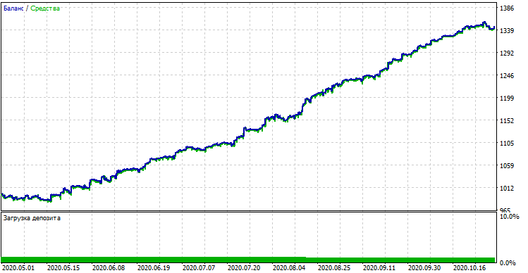
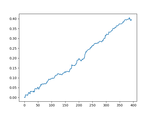
Model performance (training + validation subsamples)
If we compare the result with that obtained in the custom tester, these results are the same, except for some spread deviations. Now, let us test the model using absolutely new data, from the beginning of the year:
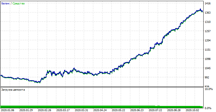
Model performance on new data
The model performed significantly worse on new data. Such a bad result is related to objective reasons, which I will try to describe further.
From Naive Models to Meaningful Ones (Further Research)
The article titled states that we are using "The Naive Approach". It is naive for the following reasons:
- The model does not include any prior data on patterns. Identifying of any patters is fully performed by gradient boosting, whose possibilities are however limited.
- The model uses a random sampling of deals, so the results in different training cycle can be different. This is not only a disadvantage but can also be considered an advantage as this feature enables the brute force approach.
- No characteristics of the general population are known in training. You never known how the model will behave with new data.
Possible ways to improve model performance (to be covered in a separate article):
- Selecting models by some external criterion (for example, performance on new data)
- New approaches to data sampling and model training, classifier stacking
- Selection of features of a different nature, based on a priori knowledge and/or assumptions
Conclusion
This article considers the excellent machine learning model entitled CatBoost: we have discussed the main aspects related to the model setup and binary classification training in time series forecasting problems. We have prepared and tested a model, as well as ported it to the MQL language as a ready-made robot. Python and MQL applications are attached below.
Translated from Russian by MetaQuotes Ltd.
Original article: https://www.mql5.com/ru/articles/8642
Warning: All rights to these materials are reserved by MetaQuotes Ltd. Copying or reprinting of these materials in whole or in part is prohibited.
This article was written by a user of the site and reflects their personal views. MetaQuotes Ltd is not responsible for the accuracy of the information presented, nor for any consequences resulting from the use of the solutions, strategies or recommendations described.
 Using cryptography with external applications
 Price series discretization, random component and noise
- Free trading apps
- Over 8,000 signals for copying
- Economic news for exploring financial markets
You agree to website policy and terms of use
prices.dropna()It didn't work at the end. The archive still contained Nan values. It was solved by simply deleting lines.
I seem unable to reproduce the results from the python tester. The MT5 tester is not reproducing the results for the same period in python tester.
Otherwise, I ported the model as explained.
I put cat_model.mqh and cat_trader.mql5(compiled to .ex5).
But results look different.
Here you can see the code for the model. Take note of MA_Period, Look_Back, etc. Then Look at the python code tester profit curve. Then look at the MT5 inputs, settings and strategy tester results.
I seem unable to reproduce the results from the python tester. The MT5 tester is not reproducing the results for the same period in python tester.
Otherwise, I ported the model as explained.
I put cat_model.mqh and cat_trader.mql5(compiled to .ex5).
But results look different.
Hello, there may be a difference between how the model was parsed when the article was written and how it happens now. CatBoost could have changed the code logic of the final model in the new versions, so you'll have to figure it out.
It seems to me that there is a high probability that this could be a problem.
I've made a few changes:
I changed the code to save the mqh according to the chart time of the data.
I changed the mqh to be different for each timeframe, so that it's possible to have all the timeframes trained and ready to use in the EA.
I changed the EA to use all the trained files for analysing and generating signals.
All the files are attached for your perusal, if possible.
If you could improve the code I would be grateful.
The strategy and also the model training need extreme improvement, if possible I appreciate help.
I've made a few changes:
I changed the code to save the mqh according to the graphical time of the data.
changed the mqh to be different for each chart time, so that all chart times can be trained and ready to use in the EA.
I changed the EA to use all the trained files for analysing and generating signals.
I have attached all the files for you to analyse if possible.
if you can improve the code i would be grateful.
the strategy and also the training of the model needs extreme improvement, if possible help thanks.