Intrinsic Time: From the Directional-Change Scaling Laws to the Alpha Engine

MetaTrader 5 — Trading | 1 October 2026, 12:10

1 041

Muhammad Minhas Qamar

Introduction

Almost everything we build in MetaTrader is clocked by the calendar. A bar closes every minute, every hour, every day, and our indicators, our models, and our Expert Advisors all sample the market on that fixed grid. But the market does not know what a minute is. During a news release a hundred meaningful moves can happen in a single minute, while over a quiet weekend an hour carries no information at all. Sampling on the clock spends the same attention on both, which means it oversamples noise and undersamples the events that actually move price.

There is an old alternative, rediscovered and formalised by the Olsen group in Zurich: let the price itself decide when time passes. In this intrinsic time, the clock ticks only when the price does something worth noticing, namely a directional change of a chosen size. This single idea turns out to be remarkably productive. The original study reports a set of empirical scaling laws that hold for close to three orders of magnitude and across thirteen currency pairs, and the same group later built on them a counter-trending trading model, the Alpha Engine, which they report is profitable even on a random walk.

In this article we build the full chain in pure MQL5 and test those claims on our own data. We implement the directional-change operator, reproduce the scaling laws on 17.8 million EUR/USD ticks, one pair over one six-month window, against a random walk of the same volatility, and port the Alpha Engine into an Expert Advisor, examining both its random-walk profit and its Strategy Tester run. The two source papers are Glattfelder, Dupuis and Olsen, Patterns in high-frequency FX data: discovery of 12 empirical scaling laws (Quantitative Finance, 2011), and Golub, Glattfelder and Olsen, The Alpha Engine: Designing an Automated Trading Algorithm (2017).

We will cover:

Intrinsic Time and the Directional-Change Operator

Fix a threshold, call it delta (for example 0.25%). Start in an up mode and track the highest price seen so far, the extreme. As long as new highs keep coming, nothing happens except that the extreme moves up. The moment the price falls by delta from that extreme, we register a directional change: the trend has, by our own definition, turned down. We flip to down mode, reset the extreme to the current price, and now wait for a rise of delta to turn us back up.

The confirming move of size delta is only part of the story. After a change confirms, the price usually keeps going in the new direction well beyond the delta that triggered the change. That continuation is the overshoot. A directional change plus the overshoot that follows it is one total move, and the whole price path becomes an alternating sequence of directional-change and overshoot sections. This is the dissection the papers call the coastline. Crucially, the clock advances only at these events, so a stormy hour and a sleepy hour are measured in the same currency: events (Fig. 1).

Dissecting a price path into directional-change and overshoot events

Fig. 1. A jagged price path resolved into directional-change (solid) and overshoot (dashed) sections at a fixed threshold; the intrinsic-time clock ticks only at the events.

The event condition is a single comparison against the extreme. Writing x for the current price and x_ext for the extreme, a downturn while in up mode is:

(x - x_ext) / x_ext <= -delta

and an upturn while in down mode is the mirror image with +delta. The paper presents this as its Algorithm 2, and we implement it as an online operator: one price at a time, no look-ahead, so the same operator can run unchanged offline over a stored tick history or online over a live feed. The class is CDcOS, and its whole decision lives in the Update method. Alongside detecting the change, it also splits each completed move at its extreme, recording the directional-change leg and the overshoot leg, which is what the scaling laws will measure.

//+------------------------------------------------------------------+
//| Feed one price update through the operator.                      |
//+------------------------------------------------------------------+
ENUM_DC_EVENT CDcOS::Update(const double price,const datetime time)
  {
   if(price<=0.0)
      return DC_EVENT_NONE;

//--- seed the state on the first valid price. The paper starts in up
//--- mode with x_ext = x_dc = x_0; the first change is therefore a
//--- warm-up whose overshoot is measured against this seed, one event
//--- of bias that a long series renders negligible.
   if(!m_initialized)
     {
      m_mode       =DC_MODE_UP;
      m_x_ext      =price;
      m_x_dc       =price;
      m_x_last     =price;
      m_t_ext      =time;
      m_t_dc       =time;
      m_idx        =0;
      m_idx_ext    =0;
      m_idx_dc     =0;
      m_initialized=true;
      return DC_EVENT_NONE;
     }

//--- drop ticks that repeat the last registered price.
   if(price==m_x_last)
      return DC_EVENT_NONE;

   m_idx++;
   m_x_last=price;
   m_event.type=DC_EVENT_NONE;

   if(m_mode==DC_MODE_DOWN)
     {
      if(price<m_x_ext)
        {
         m_x_ext  =price;               // the low runs lower: overshoot grows
         m_t_ext  =time;
         m_idx_ext=m_idx;
        }
      else if((price-m_x_ext)/m_x_ext>=m_delta)
        {
         FillEvent(DC_EVENT_UPTURN,price,time);
         Accumulate();
         m_x_dc  =price;                // reset the reference to here
         m_x_ext =price;
         m_t_dc  =time;
         m_t_ext =time;
         m_idx_dc =m_idx;
         m_idx_ext=m_idx;
         m_mode  =DC_MODE_UP;
         return DC_EVENT_UPTURN;
        }
     }
   else
     {
      if(price>m_x_ext)
        {
         m_x_ext  =price;               // the high runs higher: overshoot grows
         m_t_ext  =time;
         m_idx_ext=m_idx;
        }
      else if((price-m_x_ext)/m_x_ext<=-m_delta)
        {
         FillEvent(DC_EVENT_DOWNTURN,price,time);
         Accumulate();
         m_x_dc  =price;
         m_x_ext =price;
         m_t_dc  =time;
         m_t_ext =time;
         m_idx_dc =m_idx;
         m_idx_ext=m_idx;
         m_mode  =DC_MODE_DOWN;
         return DC_EVENT_DOWNTURN;
        }
     }

   return DC_EVENT_NONE;
  }

The two branches are symmetric. In each, the price either extends the extreme, in which case only the overshoot bookkeeping advances, or it retraces by delta, in which case a change fires. On a change, the operator calls its private FillEvent to measure the just-completed move, then resets the reference and flips mode. Everything the scaling laws need, the count of changes and the summed sizes of the legs, is accumulated as it goes, so a bank of these operators can sweep many thresholds over one tick stream in a single pass.

That measurement is the subtle part, and it is worth seeing. At the instant a change confirms, two different moves are being described at once. The extreme still holds the high or low the price ran to since the last change, and the price on record for that last change is still available, so the move that just ended can be split cleanly at its extreme. The overshoot leg runs from the last change to the extreme, and the directional-change leg runs from the extreme to the confirming price. That second leg is at least delta long, and a little longer whenever a single tick jumps past the level. Both are recorded as signed returns, together with how many price-changing ticks and how many whole seconds each leg consumed:

//+------------------------------------------------------------------+
//| Split the move that just ended at its extreme and record it.     |
//|                                                                  |
//|  Called at the confirming price, before the reset, while x_ext   |
//|  still holds the extreme and x_dc the previous change. The       |
//|  directional-change leg runs x_ext -> confirming price and is    |
//|  the delta-sized move that just fired; the overshoot leg runs    |
//|  x_dc -> x_ext and belongs to the move now ending. Leg lengths   |
//|  come straight from the stamped indices and times.               |
//+------------------------------------------------------------------+
void CDcOS::FillEvent(const ENUM_DC_EVENT type,const double price,const datetime time)
  {
   m_event.type     =type;
   m_event.price    =price;
   m_event.time     =time;
   m_event.dc_return=(price-m_x_ext)/m_x_ext;
   m_event.os_return=(m_x_ext-m_x_dc)/m_x_dc;
   m_event.ticks_dc =m_idx-m_idx_ext;
   m_event.ticks_os =m_idx_ext-m_idx_dc;
   m_event.secs_dc  =(double)(time-m_t_ext);
   m_event.secs_os  =(double)(m_t_ext-m_t_dc);
  }

Recording the overshoot only when the next change fires is what makes the coastline measurable at all: the size of an overshoot is unknowable until its extreme is final, and that happens only once the price has turned by delta. The two stamped indices make each leg's tick and time length a subtraction rather than a second pass over the data. Three details matter later: the running sums behind the scaling laws use absolute returns; a quote that repeats the last price is skipped, so tick counts are counts of price changes; and time stamps are whole seconds, so events inside one second register zero elapsed time.

Because the operator is pure computation with no dependence on bars or history, we can validate it exactly. A short hand-built price path with a large delta produces a known sequence of events whose returns, tick counts, and elapsed seconds can be computed by hand and asserted bit-for-bit; a strictly rising ramp must produce no events at all. Both tests pass, which lets us trust the numbers the next section reports.

The Scaling Laws, Verified on Real Ticks

Once a price path is a sequence of events, we can ask how the statistics of those events change as we vary the threshold delta. The scaling-law paper reports a set of empirical scaling laws that answer exactly this. Three of them tell the whole story and can be measured from the operator alone, with no time interpolation.

The full catalogue is larger. Beyond the count of changes, the paper relates the average and cumulative size of each leg to the threshold, the average number of ticks a move contains, and the average time a move or a change takes, giving eighteen relations of which twelve are independent. The waiting-time laws need a physical clock, and therefore require interpolating price onto a fixed time grid. The laws we focus on here need only the shape of the price path. That is why the operator can measure them directly, and why they are the cleanest to reproduce on a broker's raw tick stream.

The first is the directional-change count law: the number of changes at threshold delta follows a power law,

N(delta) = (delta / C)^E

with an exponent E close to -2. In plain terms, halving the threshold produces roughly four times as many events. The second concerns the overshoot. The paper's single most useful empirical fact is that, on average, the overshoot is the same size as the threshold that defined it. The paper states it plainly:

One notable observation was that, on average, a directional change delta is followed by an overshoot omega of the same magnitude, [...] this justifies the procedure of dissecting the price curve into directional-change and overshoot segments of the same size.

Since a total move is a directional change plus its overshoot, this means the average total move is about twice the threshold. The third law is the coastline: summing the sizes of every move gives a total path length that grows as a power law of delta with an exponent near -0.94, and it is far longer than intuition suggests, which is the raw material a coastline trader harvests (Fig. 2).

Scaling-law intuition: event count and the overshoot equalling the threshold

Fig. 2. The two workhorse laws at a glance: the event count scales as roughly the inverse square of the threshold, while the average overshoot roughly matches the threshold that defined it.

To measure a law we sweep a bank of operators over a grid of thresholds, accumulate each threshold's aggregates, and fit a straight line to the log of the response against the log of delta. That is exactly the estimation the paper does with a linear model: from the fitted slope B and intercept A, the scaling-law form follows with the exponent E = B and the scale C = exp(-A/B). The heart of our fitter, an excerpt from FitPowerLaw, is a plain ordinary-least-squares that also returns an honest error bar on the exponent:

//--- slope, intercept and the scaling-law parameters.
   double B=sxy/sxx;
   double A=my-B*mx;
   r.E=B;
   r.C=(MathAbs(B)>0.0)?MathExp(-A/B):0.0;
   r.R2=(syy>0.0)?(sxy*sxy)/(sxx*syy):1.0;

//--- residual variance carries the slope's standard error.
   double ss_res=syy-B*sxy;
   if(ss_res<0.0)
      ss_res=0.0;
   if(m>2)
     {
      double s2=ss_res/(m-2);
      r.SE_E=MathSqrt(s2/sxx);
     }
   r.ok=true;
   return r;

Driving the fit is a bank of operators, one per threshold, sharing a single pass over the ticks, so a forty-threshold sweep over months of data costs one read. The operators keep only running sums, never the ticks themselves, so memory stays flat no matter how long the history.

A scaling law is a claim, and a claim needs a control. The paper benchmarks every law against a Gaussian random walk, because a pattern that a structureless walk reproduces is a property of the method, not of the market. We do the same, using ALGLIB's high-quality generator, with one change: we size the walk to our own ticks rather than borrow the paper's step, for a reason the results will make clear.

//+------------------------------------------------------------------+
//| Stream a Gaussian random walk through a bank, as the negative    |
//| control the paper uses.                                          |
//|                                                                  |
//|  The paper benchmarks every law against a GRW, x_{i+1} = x_i +   |
//|  N(0, sigma^2): a pattern the walk reproduces belongs to the     |
//|  method, not to the market. Increments are additive, one second  |
//|  apart and seeded so the run repeats. Size sigma to the market's |
//|  own per-tick volatility, or the step alone distorts the slopes. |
//|  ALGLIB's high-quality generator supplies the normal draws. The  |
//|  walk is fed straight in, never stored, so memory stays flat.    |
//+------------------------------------------------------------------+
void StreamGaussianWalk(CScalingLawBank &bank,const double x0,const double sigma,
                        const long n_ticks,const int seed,const datetime t0,const int dt_sec)
  {
   CHighQualityRandStateShell st;
   CAlglib::HQRndSeed(seed,seed*7919+1,st);

   double x=x0;
   bank.Feed(x,t0);
   for(long i=1;i<n_ticks;i++)
     {
      x+=sigma*CAlglib::HQRndNormal(st);
      if(x<=0.0)
         x=x0*1e-6;                     // additive walks cannot reach here in practice
      bank.Feed(x,t0+(datetime)(i*dt_sec));
     }
  }

We ran the sweep over 17.8 million EUR/USD real ticks from our broker's history, 2 February to 31 July 2026, pulled in fortnight-long windows with CopyTicksRange. The grid is forty log-spaced thresholds from 0.02% to 2%; a threshold joins a fit once it has produced at least thirty directional changes, which leaves the thirty-two finest (0.02% to about 0.78%), and the control is fitted on that same set. The control takes one step for each of the 17.7 million price changes in the window, with the step volatility measured from those ticks, about 1.09e-5 of the price. To reproduce the results, attach the DcOS_ScalingLaws script to a EUR/USD chart and wait until the tick history is fully synced.

Then open the fit summary it writes to the terminal's Common\Files folder. The script also fits the four secondary tick- and time-based laws, which come out near the paper's values, around +2, and prints them for completeness. The exponents are the scale-invariant fingerprint we compare against the paper's EUR/USD values. Every market fit is a near-straight line, with an R-squared of at least 0.998 and a small standard error (-1.944 +/- 0.007 for the count law), but that only says the relationship is smooth over the fitted range: steadily rising or falling aggregates look straight on log-log axes almost regardless. That is why the control matters.

Law	Market exponent E	Paper (EUR/USD)	Matched random-walk E
Directional-change count	-1.944	-1.908	-1.974
Directional-change move	+0.990	+0.959	+0.993
Overshoot move	+0.938	+0.996	+1.017
Total move	+0.965	+0.976	+1.005
Coastline (cumulative total move)	-0.978	-0.940	-0.969

Every market exponent sits close to the paper's, with only the overshoot-move slope a little low. Two direct checks describe the dissection itself. The average overshoot is close to the threshold at fine resolutions, 1.025 times delta at a threshold of about 0.05% and 1.049 times at 0.02%, but it drifts down to about 0.74 times at 0.78%, where only a few dozen events remain. So "a total move is about twice delta" is a good approximation at fine thresholds rather than an exact identity. The average daily coastline at about 0.05% measured 3.82%, inside the paper's cross-pair range.

The control is where the result becomes humbling. The volatility-matched walk reproduces the market's exponents: count law -1.974 against -1.944, coastline -0.969 against -0.978. Other seeds move the walk's exponents by a few hundredths (count -1.94 to -2.00, coastline -0.96 to -1.00), more than any single fit's error bar, so gaps of that size are noise. A walk built with the paper's fixed step, about ten times coarser than a EUR/USD price change, gives -1.768 and -0.828, which looks like market structure; it is only the coarse step flattening the slopes, and matching the step closes the gap.

So at the thresholds and over the horizon we can measure on one broker's feed, EUR/USD scales like a random walk of the same volatility. The laws are real and reproducible, but they do not separate the market from noise, and our data cannot support the claim that they reveal hidden structure. The only departure we see, a slight negative correlation between consecutive price changes of about -0.06, is far too weak to move the exponents.

The coastline number is still striking. At a fine 0.05% resolution the price path travels several percent per day, far more than the day's net move. A trend follower sees only the net displacement between two points; a coastline trader sees the whole jagged length in between and aims to bank pieces of it. The matched control shows that this length is not special to the market, which moves the question to where it belongs: whether a particular way of trading the coastline makes money after costs, with its open positions counted. That is the question the rest of the article takes up.

The Alpha Engine: Coastline Trading

If a directional change is, on average, followed by an overshoot of the same size, then after a move of delta the price tends to travel another delta before it turns. A contrarian can exploit this: open against the move at an intrinsic event, and if the price runs further against the position, add to it at the next event, bringing the average entry closer to the market. This is cascading. When the price reverts, close the added pieces one by one at a profit, which is de-cascading (Fig. 3). Because the pieces are only ever added in fixed increments, this is not a martingale; it is a disciplined way to harvest the coastline. The paper's own conclusion is blunt about the surprising consequence:

Despite conventional wisdom, it is in fact possible to 'beat' a random walk. The Alpha Engine produces profitable results even on time series generated by a random walk [...] the procedure of translating a tick-by-tick time series into intrinsic time events skews the odds in one's favour.

The edge is combinatorial. The coastline operator sets its overshoot threshold to delta itself, so after a cascade one more step in the same direction has probability 1/e, which makes the next intrinsic event a de-cascade (price reverts) with probability 1 - 1/e, about 0.63, against roughly 0.37 for a further cascade. Over many events, trimming more often than adding turns the long coastline into a steady stream of realised profit. The word realised matters: the adds that are never trimmed stay open, and we will see shortly that they carry the other side of the ledger.

Two further ingredients make this robust rather than reckless. The first is asymmetric thresholds. In a sustained trend a symmetric operator keeps accumulating inventory on the losing side, so the engine skews its thresholds against the trend as inventory builds: it becomes reluctant to add and eager to trim. The paper motivates this through the notion of market-making indifference prices, and implements it pragmatically as three runners of increasing skew, chosen by the current inventory. While the position is small the symmetric runner drives it; past 15 units of inventory a runner with the adverse threshold widened to twice the favourable one takes over; past 30 units the ratio becomes four. The second ingredient is fractional sizing: when the thresholds are skewed, the unit that is added is subdivided, to a half and then a quarter, so the position grows in smaller, slower steps during exactly the conditions that are dangerous. Together they let the model lean into an ordinary overshoot while refusing to let a genuine trend run the inventory away.

Coastline trading: cascading into a move and de-cascading on the reversal

Fig. 3. A long agent cascades (adds) as price falls through successive intrinsic events, then de-cascades (trims at a profit) as price recovers; position size only ever increases by fixed increments.

The trading model needs a slightly richer operator than the scaling-law one. It works in log-price so a level is reached exactly when the log-return crosses the threshold, it keeps separate up and down thresholds so it can be skewed against a trend, and it emits not only the directional change (event code plus or minus 1) but also an overshoot event (plus or minus 2) each time the trend extends by a further step. These overshoot events are the extra intrinsic-time ticks the trader cascades on. The runner is CAeRunner, and its logic is a faithful translation of the reference Java, reading the bid and ask on the executable side of each move.

//+------------------------------------------------------------------+
//| Advance the runner by one quote.                                 |
//+------------------------------------------------------------------+
int CAeRunner::Run(const SAeTick &p)
  {
   if(!m_initialized)
     {
      m_initialized=true;
      m_extreme=m_reference=p.Mid();
      FindExpectedDc();
      FindExpectedOs();
      return AE_EVENT_NONE;
     }

   if(m_mode==-1)
     {
      if(p.bid>=m_expected_dc)
        {
         m_mode=1;                      // upturn confirmed
         m_extreme=m_reference=p.bid;
         FindExpectedDc();
         FindExpectedOs();
         return AE_EVENT_DC_UP;
        }
      if(p.ask<m_extreme)
        {
         m_extreme=p.ask;               // the low runs lower
         FindExpectedDc();
         if(p.ask<m_expected_os)
           {
            m_reference=m_extreme;       // one more downward overshoot tick
            FindExpectedOs();
            return AE_EVENT_OS_DOWN;
           }
        }
     }
   else
     {
      if(p.ask<=m_expected_dc)
        {
         m_mode=-1;                     // downturn confirmed
         m_extreme=m_reference=p.ask;
         FindExpectedDc();
         FindExpectedOs();
         return AE_EVENT_DC_DOWN;
        }
      if(p.bid>m_extreme)
        {
         m_extreme=p.bid;               // the high runs higher
         FindExpectedDc();
         if(p.bid>m_expected_os)
           {
            m_reference=m_extreme;       // one more upward overshoot tick
            FindExpectedOs();
            return AE_EVENT_OS_UP;
           }
        }
     }
   return AE_EVENT_NONE;
  }

Because the thresholds live in log-price, the runner never waits passively: each time the extreme moves it recomputes the exact price at which the next event would fire, so the trader always has a concrete level to rest an order at. The next directional change sits delta from the extreme, and the next overshoot tick sits one overshoot-threshold beyond the current reference; both are simply the extreme or the reference carried along by that log-distance:

//+------------------------------------------------------------------+
//| Price at which the next directional change would confirm.        |
//|  In down mode we watch for an up move of deltaUp above the       |
//|  extreme; in up mode a down move of deltaDown below it.          |
//+------------------------------------------------------------------+
void CAeRunner::FindExpectedDc(void)
  {
   if(m_mode==-1)
      m_expected_dc=MathExp(MathLog(m_extreme)+m_delta_up);
   else
      m_expected_dc=MathExp(MathLog(m_extreme)-m_delta_down);
  }

//+------------------------------------------------------------------+
//| Price at which the trend's next overshoot tick would register.   |
//+------------------------------------------------------------------+
void CAeRunner::FindExpectedOs(void)
  {
   if(m_mode==-1)
      m_expected_os=MathExp(MathLog(m_reference)-m_dstar_down);
   else
      m_expected_os=MathExp(MathLog(m_reference)+m_dstar_up);
  }

Each side of the market therefore has two candidate levels waiting. ExpectedLowerIE and ExpectedUpperIE hand back whichever is nearer below and above the current price, tagged by LowerIEType and UpperIEType as a change or an overshoot, and those two prices are where the coastline trader rests its limit orders.

The liquidity indicator. A pure contrarian is dangerous in a strong trend, where it cascades into an ever-larger losing position. The Alpha Engine's defence is an information-theoretic gauge of how normal the current price action is, the liquidity indicator L. It treats each intrinsic event as a symbol and measures its surprise, the self-information of the transition, then standardises the running average of surprise against its theoretical mean and variance and maps it through the normal cumulative distribution:

L = 1 - Theta( sqrt(K) * (surprise - H1) / sqrt(H2) )

Here Theta is the standard normal cumulative distribution, the surprise term is a running exponential moving average of the per-event surprise rather than a raw reading, and K is the span that sets both the standardising factor and the smoothing weight (we use 50). H1 is the entropy of the two-state directional-change/overshoot process and H2 the matching spread term, a variance in the reference's own form, with the transition probability fixed by the paper's choice of overshoot threshold, delta-star = 2.525729 times delta. When the price behaves like a normal market, L sits near 1; when the trajectory is unusually one-sided, L falls toward 0. The trader uses it to shrink its unit size in stressed conditions.

One fidelity note belongs here, as with the H2 sign below. The reference's local liquidity class computes exp(-2/(K+1)), the per-event decay factor of a span-K moving average, but multiplies the newest surprise by it rather than the running average. With K = 50 the latest event gets exp(-2/51), about 0.96, of the weight, where a conventional span-50 average would give it 2/51, about 0.04. Its global liquidity class uses the conventional ordering, so the local one looks swapped. The indicator is therefore highly reactive despite its nominal span: L behaves almost like a one-bit flag, near 0.98 after a directional change and near 0 after an overshoot step. We keep it exactly, as with its other quirks. The two moments and the per-event update read directly off the paper:

//+------------------------------------------------------------------+
//| Update the indicator on a new quote and return L.                |
//+------------------------------------------------------------------+
double CAeLocalLiquidity::Computation(const SAeTick &p)
  {
   int event=Run(p);
   if(event!=AE_EVENT_NONE)
     {
      double surprise=(MathAbs(event)==1)?0.08338161:2.525729;
      m_surp=m_alpha_weight*surprise+(1.0-m_alpha_weight)*m_surp;
      m_liq =1.0-AeCumNorm(MathSqrt(m_alpha)*(m_surp-m_h1)/MathSqrt(m_h2));
     }
   return m_liq;
  }

The two constants are the self-information of each event type: a directional change is common, so its surprise is small (0.0834), while an overshoot step is rarer, so it carries more (2.5257). The standardising constants H1 and H2 are computed once, from the transition probability alone. Note that the liquidity indicator runs on its own, wider overshoot threshold: where the cascade logic registers an overshoot every delta, this indicator registers one only every 2.525729 times delta. With that threshold, the probability that the trend takes one more overshoot step rather than reversing is exp(-2.525729), about 0.08, and from that single number the entropy and its second moment follow:

//+------------------------------------------------------------------+
//| Theoretical mean H1 and variance H2 of the per-event surprise.   |
//|  H1 is the Shannon entropy of the two-state transition; H2 is    |
//|  its second moment less H1^2 - see the fidelity note above for   |
//|  the sign the reference uses on the second term.                 |
//+------------------------------------------------------------------+
void CAeLocalLiquidity::ComputeH1H2(void)
  {
   double p=MathExp(-m_delta_star/m_delta);
   double lp=MathLog(p);
   double lq=MathLog(1.0-p);
   m_h1=-p*lp-(1.0-p)*lq;
   m_h2=p*lp*lp-(1.0-p)*lq*lq-m_h1*m_h1;
  }

The figure 2.525729 is not arbitrary: the paper chooses it to maximise the variability of the indicator, so that L separates normal from abnormal action as sharply as possible. One subtlety worth flagging: the reference computes the second moment with a sign on the second term that differs from the textbook variance, so strictly its H2 is a variance-like normaliser. We measured the cost rather than assume it: the flipped term is about 0.006, giving an H2 of 0.426 against a textbook 0.439 and moving L just after a directional change from 0.981 to 0.983. That is small enough that we keep the reference's value and flag it, rather than silently correct it.

The reference coastline trader. The runner and the liquidity indicator are only the senses; the decisions live in CAeCoastlineTrader, a faithful offline port of the paper's coastline trader that stays in the project as the reference implementation the live agent is derived from. One agent trades a single side at one base threshold. It owns a list of open cascade orders, the imbalanced list, and on every quote it rests a buy and a sell limit at the runner's two intrinsic-event levels: a fill that runs against the position is a cascade and joins the imbalanced list, a fill that runs in its favour is a de-cascade and trims it.

The inventory-aware skew is built from three runners, the construction the earlier discussion described. The symmetric runner drives a small position; once the inventory crosses 15 and then 30 units the agent hands over to runners whose adverse threshold is twice, then four times, the favourable one:

//+------------------------------------------------------------------+
//| The symmetric runner and the two inventory-skewed runners.       |
//+------------------------------------------------------------------+
void CAeCoastlineTrader::InitiateRunners(void)
  {
   double d=m_original_delta;
   m_runners[0].Init(d,d,d,d);
   if(m_long_short==1)
     {
      m_runners[1].Init(0.75*d,1.50*d,0.75*d,0.75*d);
      m_runners[2].Init(0.50*d,2.00*d,0.50*d,0.50*d);
     }
   else
     {
      m_runners[1].Init(1.50*d,0.75*d,0.75*d,0.75*d);
      m_runners[2].Init(2.00*d,0.50*d,0.50*d,0.50*d);
     }
  }

For a long agent, widening the down threshold relative to the up one makes it slower to add as the price keeps falling and quicker to trim as it recovers; the short agent is the mirror image. The paper's prose describes this skew the opposite way round from its own reference code; the economics are the same, and we follow the code. The same arithmetic configures the live EA's runners in the next section, so the skew is part of the shared decision core.

The de-cascade is where the accounting lives. When the price reverts, a trim does not merely shrink a net position; it compensates a specific set of open cascade orders, the ones it can now close at a profit. That set is every order in the imbalanced list the trim clears by at least delta:

//+------------------------------------------------------------------+
//| Collect the open orders a trim at 'level' would profitably close.|
//+------------------------------------------------------------------+
void CAeCoastlineTrader::FindCompensatedOrdersList(const double level,const double delta,const int buy_sell,CAeLimitOrder *&out[])
  {
   ArrayResize(out,0);
   int n=ArraySize(m_imbalanced);
   for(int i=0;i<n;i++)
     {
      double lvl=m_imbalanced[i].Level();
      if((lvl-level)*buy_sell>=delta*lvl)
        {
         int k=ArraySize(out);
         ArrayResize(out,k+1);
         out[k]=m_imbalanced[i];
        }
     }
  }

The trim then takes its own size from the orders it compensates and books their combined profit at its level, each compensated add earning the distance the price travelled back in its favour, expressed as a return and scaled by the add's size:

//+------------------------------------------------------------------+
//| Realised profit of closing the compensated orders here.          |
//|  For each compensated order, the price moved (level - this.level)|
//|  in this order's favour, expressed as a return on the compensated|
//|  level and scaled by its volume.                                 |
//+------------------------------------------------------------------+
double CAeLimitOrder::RelativePnL(void) const
  {
   double pnl=0.0;
   int n=ArraySize(m_compensated);
   for(int i=0;i<n;i++)
     {
      double abs_move=(m_compensated[i].Level()-m_level)*m_type;
      pnl+=abs_move/m_compensated[i].Level()*m_compensated[i].Volume();
     }
   return pnl;
  }

A position closes for good once its total return, the realised de-cascade profit plus the open mark-to-market, reaches the trader's own delta. The reference leaves this profit target as a stub; following the author's overview code we set it to delta of return on the size the position opened with, and check it on every quote:

//+------------------------------------------------------------------+
//| Take-profit target for a freshly opened position.                |
//|  The reference stubs this; following its overview code, the      |
//|  target is delta of return on the size the position opened with. |
//+------------------------------------------------------------------+
void CAeCoastlineTrader::ComputeTargetPnL(CAeLimitOrder *opening)
  {
   m_target_pnl=m_original_delta*opening.Volume();
  }

Profit on a random walk. The paper's boldest claim can be tested with no market data at all. We stream seeded Gaussian random walks through the full eight-agent engine and read the profit two ways, kept strictly apart from here on: realised profit counts closed round trips only, and total profit adds the mark-to-market of whatever cascade is still open at the final tick. Across two hundred walks of a million ticks each, the realised profit was positive every single time, averaging +4.33 in the engine's abstract return units: the 1 - 1/e trimming asymmetry books more de-cascades than cascades even in pure noise, exactly as the paper describes.

The total profit tells a different story. The open cascade averaged -4.12, and the total +0.22 with a standard error of 0.36, indistinguishable from zero. The typical walk still finishes ahead, 123 of the 200 with a median of +1.58, but the losers lose large, the worst near -17. This is what theory predicts: on a random walk with no drift, no rule that sees only past prices can have a positive expected total profit. The dissection reshapes the payoff into many small realised gains and occasional large open losses, so the paper's claim holds for realised profit.

Random-walk PnL (200 seeds, 1M ticks each)	Profitable seeds	Mean	Median	Worst seed
Realised (closed round trips)	200/200	+4.33	+4.34	+1.78
Total (incl. open mark-to-market)	123/200	+0.22	+1.58	-17.18

This distinction is the lens for the rest of the article: closed trades will almost always look good, and whether there is an edge is decided by what is still being held.

This offline trader is the fidelity anchor for the whole port: a literal translation of the reference, checked by a known-answer self-test, and the random-walk figures above come from the attached Ae_RandomWalk script driving it. The live Expert Advisor in the next section keeps its runners and liquidity indicator verbatim and adapts the execution in two places: how a de-cascade is carried out once real hedged positions replace the imbalanced list, and, as we flag there, the reference's whole-position exit, which the live agent does not reproduce.

Building the Expert Advisor

The reference trades in abstract units against a price feed; the live agent must move real lots. Following the paper's insistence on limit orders, it runs the entire lifecycle in limit orders on a hedging account, where each cascade step is naturally its own position.

The mapping is clean. A long agent keeps a single buy-limit resting at the next downward intrinsic-event level, and each fill opens a position with a take-profit exactly delta above its entry. That take-profit is the de-cascade: as the price falls, the ladder of buy-limits fills and the position cascades; as it recovers, the take-profits trim it one by one. A short agent is the mirror image.

Limit orders remove slippage, not the spread. A buy-limit fills when the ask reaches its level and its take-profit when the bid reaches the target, so the booked profit is level to level but the price must travel delta plus the spread for each round trip. The per-tick logic of one agent, CAeLiveTrader, is:

//+------------------------------------------------------------------+
//| Drive the agent one quote forward.                               |
//+------------------------------------------------------------------+
void CAeLiveTrader::OnTickUpdate(const double bid,const double ask,const datetime time)
  {
   SAeTick t=AeTick(bid,ask,time);
   m_liq.Computation(t);

   int ev[3];
   ev[0]=m_runners[0].Run(t);
   ev[1]=m_runners[1].Run(t);
   ev[2]=m_runners[2].Run(t);

   double inv=InventoryUnitsAbs();
   int idx=ProperRunnerIndex(inv);

//--- safety cap: stop adding once the inventory is large; the resting
//--- take-profits still unwind what is open.
   if(inv>=m_max_units)
     {
      CancelEntry();
      m_last_idx=idx;
      return;
     }

//--- re-place the entry only when something changed: an intrinsic
//--- event on the active runner, a tier switch, or no order resting.
   bool refresh=(ev[idx]!=AE_EVENT_NONE) || (idx!=m_last_idx) || (MyEntryTicket()==0);
   m_last_idx=idx;
   if(!refresh)
      return;

   double unit=UnitFromInventory(inv);
   double vol_units=unit*LiqCoef(m_liq.Liq());
   double lots=NormalizeLots(vol_units*m_lot_per_unit);
   if(lots<m_lot_min)
      return;

   double level,tp;
   if(m_long_short==1)
     {
      level=m_runners[idx].ExpectedLowerIE();
      tp=level*(1.0+m_delta);
      if(ask-level<=m_stop_dist)          // too close to place a buy limit
         return;
     }
   else
     {
      level=m_runners[idx].ExpectedUpperIE();
      tp=level*(1.0-m_delta);
      if(level-bid<=m_stop_dist)          // too close to place a sell limit
         return;
     }

   PlaceOrRefreshEntry(level,lots,tp);
  }

The volume rules are the paper's, mapped to lots by a LotPerUnit input: the base unit is halved then quartered as inventory crosses 15 and 30 units, and shrunk again by the liquidity coefficient. Three runners are advanced on every tick, but only the one selected by the current inventory drives the orders, which is how the inventory-driven threshold skew takes effect. The entry is only re-placed when it needs to move, on an intrinsic event, a tier switch, or after a fill, so the EA is not churning orders on every tick.

Placing and maintaining that single resting order is the job of PlaceOrRefreshEntry. If none of our orders rests, it sends a fresh buy-limit or sell-limit carrying the take-profit. If one already rests but the desired size has changed, and a pending order's volume cannot be modified in place, it deletes and re-sends; otherwise, if only the level or the take-profit has drifted, it nudges them with a single modify. The effect is that each agent always has exactly one entry alive, sitting at the current intrinsic-event level with its de-cascade exit already attached:

//+------------------------------------------------------------------+
//| Put a limit entry at 'level' with take-profit 'tp', or update    |
//| the resting one if the level, take-profit or size has moved.     |
//+------------------------------------------------------------------+
void CAeLiveTrader::PlaceOrRefreshEntry(const double level,const double lots,const double tp)
  {
   double lvl=NormalizeDouble(level,m_digits);
   double take=NormalizeDouble(tp,m_digits);

   double cur_lvl,cur_vol,cur_tp;
   if(!MyEntryInfo(cur_lvl,cur_vol,cur_tp))
     {
      if(m_long_short==1)
         m_trade.BuyLimit(lots,lvl,m_symbol,0.0,take,ORDER_TIME_GTC,0,"AE");
      else
         m_trade.SellLimit(lots,lvl,m_symbol,0.0,take,ORDER_TIME_GTC,0,"AE");
      return;
     }

//--- volume cannot be modified on a pending order: replace it.
   if(MathAbs(cur_vol-lots)>=m_lot_step*0.5)
     {
      ulong tk=MyEntryTicket();
      if(tk!=0)
         m_trade.OrderDelete(tk);
      if(m_long_short==1)
         m_trade.BuyLimit(lots,lvl,m_symbol,0.0,take,ORDER_TIME_GTC,0,"AE");
      else
         m_trade.SellLimit(lots,lvl,m_symbol,0.0,take,ORDER_TIME_GTC,0,"AE");
      return;
     }

//--- otherwise nudge the level / take-profit if they drifted.
   if(MathAbs(cur_lvl-lvl)>=m_point || MathAbs(cur_tp-take)>=m_point)
     {
      ulong tk=MyEntryTicket();
      if(tk!=0)
         m_trade.OrderModify(tk,lvl,0.0,take,ORDER_TIME_GTC,0);
     }
  }

One design decision deserves a word on fidelity. In the reference, a de-cascade is a limit order that reduces the net position, a netting-account idea. On a hedging account each cascade position instead carries its own take-profit at delta, and the two are closer than they look: the FindCompensatedOrdersList test above, run with the original delta, closes an order once the trim level is at least delta beyond the order's own level, which is exactly a take-profit at delta. The difference is timing. The reference trims only at its next intrinsic-event level, at or beyond that target, while the live agent closes each position the moment its target is touched, slightly earlier and slightly smaller. The decision core, the runners and the liquidity indicator, is the verbatim port.

There is a second, more consequential difference. The reference also has a whole-position exit: once a position's total return, realised plus open, reaches delta, it closes everything at market. The live agent does not reproduce it. MaxUnits still caps the inventory, but a cascade that runs adverse and never recovers is only halted, not closed, with its take-profits left resting. This is the single largest risk in the live design, and the backtest in the next section shows what it costs.

A practical caveat comes with mapping abstract units to lots. The paper's fractional sizing produces adds as small as a quarter of a unit scaled by the liquidity coefficient, and on a broker with a 0.01-lot step those only survive as distinct sizes when LotPerUnit is large enough, around 0.4, that the smallest add still clears the minimum lot. Below that, the smaller adds are raised to the minimum lot and the fine sizing collapses onto fewer sizes, although the more important threshold skew, which lives in the runners rather than in the volume, is unaffected.

The top-level Expert Advisor is the ensemble the paper specifies: eight agents, a long-only and a short-only one at each of four thresholds, 0.25%, 0.5%, 1%, and 1.5%. Each agent owns its orders and positions through a unique magic number. Because the whole design depends on independent positions, the EA refuses to run on anything but a hedging account:

//+------------------------------------------------------------------+
//| Enforce a hedging account and build the requested agents.        |
//+------------------------------------------------------------------+
int OnInit(void)
  {
   long mode=AccountInfoInteger(ACCOUNT_MARGIN_MODE);
   if(mode!=ACCOUNT_MARGIN_MODE_RETAIL_HEDGING)
     {
      Print("AlphaEngine: a hedging account is required "
            "(each cascade step must be its own position). Aborting.");
      return INIT_FAILED;
     }

   if(InpLotPerUnit<=0.0 || InpMaxUnits<=0.0)
     {
      Print("AlphaEngine: LotPerUnit and MaxUnits must be positive.");
      return INIT_FAILED;
     }

   g_count=0;
   for(int s=0;s<4;s++)
     {
      if(InpTradeLong)
        {
         g_traders[g_count].Init(_Symbol,InpMagicBase+s*2,1,
                                 g_deltas[s],InpLotPerUnit,InpMaxUnits);
         g_count++;
        }
      if(InpTradeShort)
        {
         g_traders[g_count].Init(_Symbol,InpMagicBase+s*2+1,-1,
                                 g_deltas[s],InpLotPerUnit,InpMaxUnits);
         g_count++;
        }
     }

   if(g_count==0)
     {
      Print("AlphaEngine: no agents enabled.");
      return INIT_FAILED;
     }
   PrintFormat("AlphaEngine: %d agents live on %s (hedging).",g_count,_Symbol);
   return INIT_SUCCEEDED;
  }

One practical detail matters for a clean run. Outside trading hours the terminal rejects order operations as "market closed", and eight agents each retrying at every session boundary floods the journal and slows a long backtest to a crawl. A small helper, InTradeSession, checks the symbol's session table with SymbolInfoSessionTrade and lets OnTick return early when the market is shut. This is almost certainly harmless, since there are essentially no ticks while the market is closed, though strictly it does mean the runners do not update outside a session; it keeps the run fast and the journal readable:

//+------------------------------------------------------------------+
//| Is the symbol inside a trading session right now.                |
//|  Order operations outside a session are rejected as "market      |
//|  closed"; gating on the session keeps the journal clean and the  |
//|  run fast. The runners also pause outside a session, which only  |
//|  matters if the feed keeps quoting while trading is closed.      |
//+------------------------------------------------------------------+
bool InTradeSession(void)
  {
   MqlDateTime st;
   TimeToStruct(TimeCurrent(),st);
   ENUM_DAY_OF_WEEK dow=(ENUM_DAY_OF_WEEK)st.day_of_week;
   uint sod=(uint)(st.hour*3600+st.min*60+st.sec);
   datetime from,to;
   for(uint s=0;SymbolInfoSessionTrade(_Symbol,dow,s,from,to);s++)
      if(sod>=(uint)from && sod<(uint)to)
         return true;
   return false;
  }

//+------------------------------------------------------------------+
//| Drive every agent with the freshest quote.                       |
//+------------------------------------------------------------------+
void OnTick(void)
  {
   if(!InTradeSession())
      return;

   MqlTick t;
   if(!SymbolInfoTick(_Symbol,t))
      return;
   if(t.bid<=0.0 || t.ask<=0.0)
      return;

   for(int i=0;i<g_count;i++)
      g_traders[i].OnTickUpdate(t.bid,t.ask,t.time);
  }

Running the ensemble is a matter of attaching it to a EUR/USD chart on a hedging account, or loading it in the Strategy Tester with the Every tick based on real ticks model. One practical trap: the Strategy Tester inherits the margin mode of the account you are logged into, so a reader on a netting account will see the EA abort with INIT_FAILED by design; log into a hedging account before testing. Its inputs are deliberately few:

Input	Meaning
InpLotPerUnit	Lots per one abstract unit. Raise it toward 0.4 to keep the fractional sizing exact on a 0.01-lot symbol, or lower it to trade smaller.
InpMaxUnits	Per-agent inventory cap, in units. Once reached, no new adds are placed and the open take-profits are left to unwind the position.
InpMagicBase	Base magic number. Each of the eight agents takes a distinct magic derived from it, so they never touch each other's orders.
InpTradeLong / InpTradeShort	Enable the four long-only and the four short-only agents independently; both are on by default for the full symmetric ensemble.

Strategy Tester Results

We tested the ensemble on EUR/USD in the Strategy Tester using the Every tick based on real ticks model, the same broker data behind the scaling-law study, over roughly six months (2 February to 31 July 2026) and starting from a 10,000 deposit on a hedging account. The run used the shipped defaults, LotPerUnit = 0.02 and MaxUnits = 30, with all eight agents enabled. The tester journal shows the mechanism working as designed: buy-limits triggering in a descending ladder as the price falls, and take-profits firing as the price recovers. Not every cascade unwound on its own, though. When the test ended, 24 positions from cascades that had not recovered were still open, and the tester closed them at the final price.

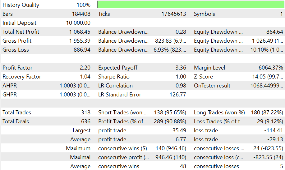
Strategy Tester report for the Alpha Engine on EUR/USD

Fig. 4. The Strategy Tester report tab for the six-month EUR/USD run.

A single window into the journal behind that report (Fig. 4) makes the lifecycle concrete. During one decline the long agent at the 0.25% threshold filled buy-limits in a descending ladder, at 1.17901, then 1.17898, then lower, each opening its own position with a take-profit set delta above its fill. As the price turned back up, those take-profits triggered in turn, for instance closing a position bought near 1.17832 at its target, banking a small profit and reducing the inventory by one step. Entries and exits are both limit fills at levels fixed in advance, which is the practical payoff of clocking the model on intrinsic events rather than on the raw tick.

In MetaTrader every position is opened and later closed by two deals, so the 637 deals track the 318 positions the agents opened and closed over the run, plus the initial balance entry. The net figure hides two very different streams, and splitting it by how each position closed is more instructive than the total:

Component of the six-month result	Amount
294 positions closed at their take-profit	+1,934.14
24 positions closed by the tester at the end of the run	-823.55
Commission charged on entries	-42.14
Net profit	+1,068.45

Both closing lines already include swap, which came to -620.38. The tester's final close gave back 824: that is the missing whole-position exit showing up in the numbers, the cascades that never recovered. And swap, the overnight financing of held positions, cost far more than commission and turned five take-profit trades into net losses. For a model that can hold a cascade for weeks, financing, not the spread, is the dominant cost.

The 10.68% comes from one pair over one six-month window, so it shows a working mechanism rather than a headline performance number, and it is not comparable to the paper's 21.34%, an eight-year result across twenty-three pairs. The curves in Fig. 5 show the same split as the table. The balance, which moves only when a position closes, climbs in small steps; the equity, which marks the open cascades, swings below it and meets it only at the final-day drop. A rising balance is what any strategy that closes winners and holds losers produces, so it is not in itself evidence of an edge.

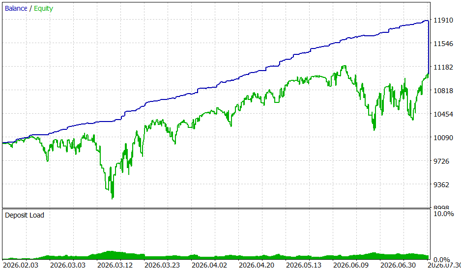
Equity and balance curve of the Alpha Engine backtest

Fig. 5. The balance (blue) steps up as take-profits fire; the equity (green) carries the open cascades and meets the balance only when the tester closes them on the last day.

Because a short window can flatter a strategy that trades infrequently, it helps to see the same EA over three lengths of the same period. On a two-week window there are too few complete cascade-and-unwind cycles for the profit factor to mean much, and it reads implausibly high; as the window lengthens and hundreds of cycles accumulate, the profit factor settles near 2.2 and the drawdown grows with the time the capital is exposed.

Test window	Return	Trades	Profit factor	Max equity DD
Two weeks	+1.21%	22	45.48	0.35%
Two months	+2.14%	70	2.71	3.17%
Six months	+10.68%	318	2.21	10.10%

None of this is an optimisation result: the thresholds, the sizing rules, and the take-profit are the paper's, not tuned to this symbol or period. What the tester shows is narrower than an edge. The live agent runs the mechanism through real spreads, swap and session gaps, and it finished this window positive after costs and after the forced close. One pair and one period cannot establish an edge, and the random walk shows that steady realised wins can coexist with none. Annualised, the run makes far more than the paper's 21.34% over eight years, but at about 10% drawdown against their 0.71%, which is what one pair with no diversification and no whole-position exit should look like.

NOTE: The results use the shipped defaults, LotPerUnit = 0.02 and MaxUnits = 30, so the backtest runs a simplified version of the paper's sizing. At 0.02 lots per unit a full add is 0.02 lots and every smaller add, the half and quarter units and any add cut by the liquidity haircut, is raised to the 0.01-lot minimum. The sizing therefore has two steps instead of the paper's ladder, and the liquidity indicator, which behaves almost as a one-bit flag, only switches a full add between 0.02 and 0.01 lots; raising LotPerUnit toward 0.4 restores the ladder. And since the deepest skew tier engages only past 30 units, a MaxUnits of 30 means it is never reached unless the cap is raised.

Conclusion

We took a single idea, that time in markets is better measured in events than in seconds, and followed it all the way from a definition to a working Expert Advisor. Along the way we:

Built the directional-change operator that dissects a tick stream into directional-change and overshoot events, validated bit-for-bit against a hand-computed path.
Reproduced the empirical scaling laws on 17.8 million real EUR/USD ticks, matching the paper's exponents closely, and showed with a volatility-matched random walk that, at these scales, the same laws hold for pure noise.
Ported the Alpha Engine, its log-threshold runner, its information-theoretic liquidity indicator, and its cascading and de-cascading logic, staying faithful to the reference including the quirks we chose not to patch.
Delivered a working Expert Advisor that trades the model with limit orders on a hedging account and, in a six-month real-tick backtest, returned 10.68% on the deposit with a profit factor of 2.21 and a 10.10% equity drawdown, after swap, commission and the tester's closing of the positions still open at the end.

The most instructive result is the random walk. Clocked by intrinsic time, a bare-bones contrarian books realised profit on every one of 200 random walks, yet its total profit, open inventory included, averages zero. The event-based view skews the odds of each trim in the trader's favour, but it reshapes the payoff rather than creating an edge, and that is the lens for reading any coastline trader's results, our own backtest included. The natural next steps are cost and swap sensitivity, more pairs and periods, and a proper risk layer, above all a whole-position exit for the live agent, and the code is written to make them straightforward.

The programs presented in this article are intended for educational purposes only. Trading carries a high level of risk, and past performance, especially on historical data, is not indicative of future results. Always test thoroughly on a demo account before risking capital.

Getting the Source Code via MQL5 Algo Forge

All source files are attached to this article below, but the full repository is also available on MQL5 Algo Forge, the community's Git-based platform for sharing and collaborating on trading projects.

File name	Description
MQL5\Include\IntrinsicTime\DcTypes.mqh	Shared enums and the directional-change event record
MQL5\Include\IntrinsicTime\DcOperator.mqh	CDcOS, the directional-change / overshoot dissection operator
MQL5\Include\IntrinsicTime\ScalingLaws.mqh	Operator bank, log-log power-law fit, and the random-walk control
MQL5\Include\IntrinsicTime\AeTypes.mqh	Tick structure and intrinsic-event codes for the trading model
MQL5\Include\IntrinsicTime\AeRunner.mqh	CAeRunner, the log-threshold runner emitting DC and overshoot events
MQL5\Include\IntrinsicTime\AeLiquidity.mqh	CAeLocalLiquidity, the information-theoretic liquidity indicator L
MQL5\Include\IntrinsicTime\AeLimitOrder.mqh	Reference limit-order record with de-cascade profit accounting
MQL5\Include\IntrinsicTime\AeCoastlineTrader.mqh	The offline reference coastline trader used to validate the port
MQL5\Include\IntrinsicTime\AeAlphaEngine.mqh	The eight-agent ensemble in offline reference form
MQL5\Include\IntrinsicTime\AeLiveTrader.mqh	CAeLiveTrader, one live coastline agent trading real limit orders
MQL5\Scripts\IntrinsicTime\DcOS_SelfTest.mq5	Known-answer tests for the directional-change operator, plus a real-tick probe
MQL5\Scripts\IntrinsicTime\DcOS_ScalingLaws.mq5	Streams historical real ticks and a random walk, fits every law, dumps the results
MQL5\Scripts\IntrinsicTime\Ae_SelfTest.mq5	Known-answer tests for the runner, order accounting, and a round trip
MQL5\Scripts\IntrinsicTime\Ae_RandomWalk.mq5	Runs the reference engine over seeded random walks and reports the profit distribution
MQL5\Experts\IntrinsicTime\AlphaEngine.mq5	The Expert Advisor: the eight-agent Alpha Engine for a hedging account

Attached files |

Download ZIP

MQL5.zip (38.51 KB)

Warning: All rights to these materials are reserved by MetaQuotes Ltd. Copying or reprinting of these materials in whole or in part is prohibited.

This article was written by a user of the site and reflects their personal views. MetaQuotes Ltd is not responsible for the accuracy of the information presented, nor for any consequences resulting from the use of the solutions, strategies or recommendations described.