Implementing and Comparing Five Historical Volatility Estimators in MQL5

Introduction

Historical volatility is not a single calculation. The five estimators use closing prices, the high–low range, or the complete OHLC tuple and encode different assumptions. Applying the generic label “historical volatility” without identifying the estimator can therefore conceal a material implementation choice.

This study compares five historical volatility estimators: Close-to-Close, Parkinson, Garman-Klass, Rogers-Satchell, and Yang-Zhang. The practical question is deliberately narrow:

Each rolling variance estimate is carried forward unchanged as a one-session-ahead persistence forecast. How do the five estimators rank against the next broker D1 session's M1 realized-variance proxy for EURUSD, and is the main Parkinson–Yang-Zhang QLIKE difference distinguishable from zero?

The implementation includes a reusable include module, a chronological comparison script, a deterministic validation script, a robustness script, and a configurable indicator. Detailed, summary, session-audit, paired circular moving-block bootstrap, and past-only rolling scale calibration CSV files are also provided. These components let MQL5 developers reproduce the workflow and verify the formulas, chronology, target construction, and reported comparisons.

The main comparison uses a 20-session D1 estimation window for EURUSD. The 10-session and 40-session windows are declared sensitivity settings.

The question concerns non-annualized variance. It does not identify an estimator that should be preferred for every market, a trading signal, an option-pricing input, or a profitable strategy. EURUSD is used as one controlled case study so every estimator receives the same sessions, forecast origins, and forecast targets under one common target mask.

The single-instrument design fixes input bars, target sessions, estimation windows, and scoring rules. Only the estimator formula changes. Cross-market ranking stability and trading applications are outside this study because they require additional experimental decisions.

What the comparison measures

The following terms fix the unit of analysis before any formula or result is introduced.

• Session: one completed broker D1 bar, bounded by the broker server-time bar convention.
• Estimation window: the n completed return intervals used for one historical variance estimate.
• Variance estimate: a non-annualized value returned by one estimator at the forecast origin.
• Variance forecast: the estimate carried forward unchanged for the next session.
• Realized-variance proxy: the next session’s close-to-open squared jump plus squared returns reconstructed from chronological M1 closes.
• Forecast origin: the close of session t, when only data through that session are available.
• Forecast target: the realized-variance proxy for session t + 1.
• Common target mask: the sessions whose estimation windows and realized-variance proxies are valid for all five estimators.
• Evaluation loss: an error measure between a variance forecast and its forecast target.

The estimator and the forecast rule are separate. Each estimator summarizes the same estimation window. The experiment then applies a deliberately simple persistence rule:

h_{t+1} = sigma_hat_t^2

Here, sigma_hat_t^2 is the historical variance estimate available at the close of session t, and h_{t+1} is the raw variance forecast for the next session. This primary forecast has no fitted coefficient. A separate sensitivity check applies a rolling scale factor estimated only from the preceding 252 valid sessions.

The main estimation window is n=20. The n=10 and n=40 estimation windows are sensitivity settings. This hierarchy is a declared design choice in the supplied protocol, not an externally registered design. The three windows are not independent experiments or optimization candidates.

Case-study configuration

The reported results are actual historical script output for six complete calendar years of EURUSD forecast targets, from 2020 through 2025. This fixed interval supplies 1,560 candidate forecast targets while preserving the controlled single-instrument design.

Setting	Recorded value
Instrument	EURUSD
Evidence type	Actual historical script output
Broker environment	MetaQuotes-Demo
Target period	2020–2025
Historical input	Completed D1 OHLC bars
Forecast target	Next-session M1 realized-variance proxy
Estimation windows	n=10, n=20, n=40; main n=20
M1 coverage policy	At least 1,380 M1 bars; largest internal gap no greater than 300 seconds
D1/M1 endpoint tolerance	1e-10, scaled by the larger of one and the two absolute prices
QLIKE floor	1e-12; zero floor events in the reported run
Primary criterion	Mean QLIKE at n=20
Candidate forecast targets	1,560 completed sessions
Common target mask	1,472 retained sessions
Paired circular moving-block bootstrap	Circular moving blocks of 20 sessions; 10,000 replications; seed 260924
Past-only rolling scale calibration	Past-only rolling scale over 252 valid sessions

The broker history contained 1,560 candidate D1 target sessions: 260 in each year from 2020 through 2023, 261 in 2024, and 259 in 2025. The count comes from the D1 bars actually returned by the MetaQuotes-Demo history, not from an assumed weekday calendar.

Six weekdays had no broker D1 bar: 1 January 2020, 25 December 2020, 1 January 2021, 1 January 2024, 1 January 2025, and 25 December 2025. Each is New Year's Day or Christmas Day, and the downloaded broker history supplies no target bar for it. They are outside the 1,560 candidate sessions rather than exclusions applied by the M1 coverage policy.

The M1 coverage policy retained 1,472 sessions and excluded 88 before scoring. Of these, 42 had fewer than 1,380 M1 bars and 46 had an internal timestamp gap above 300 seconds. All five estimators use the same 1,472 sessions under every estimation window. The n=10 and n=40 calculations remain sensitivity checks.

The comparison script recreates the detailed, summary, and session-audit CSV files with FILE_WRITE on every run. Preserve or rename an earlier export before rerunning the study if it is needed for comparison. These fixed settings and retained sessions define the input sample. The data-alignment and chronological-order rules applied to that sample are defined next.

Data alignment and chronological order

The comparison uses completed EURUSD D1 bars for the historical volatility estimators and M1 bars for the next-session forecast target. The exact broker-session boundary is accepted as part of the data definition. It is not interpreted as an exchange close, and the conclusions do not require one. The same boundary is applied consistently to every estimator and forecast target.

Every calculation with an estimation window of length n requires n + 1 chronological D1 bars. The first bar provides C_{i−1}; the following n bars provide the returns being estimated. An implementation that passes only n bars either omits one return or obtains the previous close from outside the supplied estimation window.

The forecast origin is always a completed D1 close. The script never reads the current incomplete bar, and it never uses M1 observations from the target session while forming the estimate. Without this chronological separation, a mathematically correct estimator can still produce a look-ahead comparison.

CopyRates() writes the oldest copied element at the beginning of physical memory, irrespective of the logical series flag. The scripts explicitly normalize the arrays to chronological order, and the include module rejects repeated or decreasing timestamps. This validation prevents reversed series input. Without it, logarithmic returns can look plausible while encoding incorrect time order.

The script accepts a history request only when CopyRates() returns the full interval (CopyRates() == Bars()). A positive but partial response is retried. Retry diagnostics retain the current SERIES_SYNCHRONIZED state. Any incomplete M1 chunk aborts the run, preventing partial history from entering the comparison.

For each forecast target, M1 bars are sliced to the exact half-open interval:

[target_D1_time, next_D1_time)

Missing minutes are neither synthesized nor forward-filled. A forecast target is retained only when its M1 path belongs to the corresponding D1 interval, its endpoints agree with the D1 bar, and its timestamps are chronological. The detailed CSV preserves the coverage diagnostics, but all five estimators share the common target mask. If a forecast target is unavailable, it is unavailable to every estimator; availability does not depend on estimator processing order.

The common target mask removes estimator-specific sample differences: every reported mean averages the same sessions. It does not eliminate selection bias created by the broker history, the coverage rules, the chosen instrument, or the test period. Validation of the estimation window and forecast target is completed before any evaluation loss is recorded for any estimator.

In the detailed CSV, forecast origin is the close of the last completed D1 bar in the estimation window. It is computed as bar open + PeriodSeconds(PERIOD_D1). target_time is the opening time of the following available D1 forecast target. The two timestamps can differ across a weekend or another non-trading interval. This timestamp contract supplies the common chronological input used by all five historical volatility estimators.

Five historical volatility estimators

For session i, let O_i, H_i, L_i, and C_i denote open, high, low, and close. The preceding session close is C_{i−1}. The common log-price terms are:

r_i = ln(C_i / C_{i−1})
o_i = ln(O_i / C_{i−1})
c_i = ln(C_i / O_i)
u_i = ln(H_i / O_i)
d_i = ln(L_i / O_i)
x_i = ln(H_i / L_i)

All calculations below return variance, not volatility. A displayed volatility would be sqrt(variance), but square roots are not used for the forecast scores.

Close-to-Close

r_bar is the arithmetic mean of the n close-to-close returns. Close-to-Close uses closing returns, so r_i includes close-to-open movement. It discards intraday range information. The implementation uses the sample denominator n − 1.

sigma_CC^2 = [1 / (n − 1)] * sum_{i=1}^{n} (r_i − r_bar)^2

Close-to-Close requires only consecutive closing prices. Two sessions with identical previous and current closes produce the same close-to-close return irrespective of their intraday high–low ranges. Close-to-Close therefore provides a baseline for evaluating whether additional OHLC information lowers the evaluation losses for the next-session forecast.

Parkinson

Parkinson uses the high–low range. Under its idealized continuous-price assumptions, the range can contain more information than one close-to-close return. The estimator does not add a separate close-to-open jump component and does not explicitly accommodate drift.

sigma_P^2 = [1 / (4 * n * ln(2))] * sum_{i=1}^{n} x_i^2

The Parkinson formula requires only H_i and L_i. It can understate variance when the close-to-open displacement is large relative to the intraday high–low range because the previous close does not enter the formula. Data errors affecting recorded intraday highs or lows directly affect range-based estimators, whereas they do not enter a closing-return calculation unless the recorded closing price is also affected.

Garman-Klass

Garman-Klass combines the range with the open-to-close return. Its efficiency arguments rely on restrictive no-jump and drift assumptions. Those theoretical properties do not guarantee the lowest empirical evaluation loss on broker quote bars.

sigma_GK^2 = (1 / n) * sum_{i=1}^{n} [0.5 * x_i^2 − (2 * ln(2) − 1) * c_i^2]

The subtraction involving c_i^2 is not an arbitrary correction. It adjusts the range contribution using the directional movement between the session open and close. Valid OHLC ordering implies |c_i| ≤ x_i, while 2 * ln(2) − 1 < 0.5, so each displayed per-session contribution is nonnegative. Per-term clamping is unnecessary and could conceal invalid input data or a numerical failure.

Rogers-Satchell

Rogers-Satchell is drift-independent under its stated assumptions. It uses OHLC information but does not add a distinct close-to-open jump variance.

sigma_RS^2 = (1 / n) * sum_{i=1}^{n} [u_i * (u_i − c_i) + d_i * (d_i − c_i)]

Its cross-products differ structurally from the squared-range formulas. The terms compare the high and low with both the open and close, so the calculation incorporates session direction without estimating mean drift. Close-to-open movement remains outside its explicit variance component.

Yang-Zhang

sigma_o^2 is the sample variance of o_i, sigma_c^2 is the sample variance of c_i, and sigma_RS^2 is the Rogers-Satchell component over the same estimation window. Both sample variances retain denominator n − 1; the Rogers-Satchell component retains denominator n. Yang-Zhang combines opening, open-to-close, and range information to address drift and close-to-open jumps under its assumptions.

sigma_YZ^2 = sigma_o^2 + k * sigma_c^2 + (1 − k) * sigma_RS^2

k = 0.34 / [1.34 + (n + 1) / (n − 1)]

Yang-Zhang has the most complex component structure among the five estimators. Its opening returns, open-to-close returns, and Rogers-Satchell contribution must be calculated over the same sessions rather than as three independent estimation windows. The coefficient k also depends on n, so a value hard-coded for one estimation window is invalid when n changes.

The five outputs are deliberately returned together by CalculateAll(). The logarithmic transformations are shared, which reduces duplicated code and ensures that all formulas see identical prices. More importantly, the caller cannot accidentally form one estimator from a shifted estimation window while forming another from the intended one.

The complete CalculateAll() implementation below transforms each interval once, applies the estimator-specific denominators, and validates all five outputs under the same numerical convention.

//+------------------------------------------------------------------+
//| Calculate all five variance estimators from the same window      |
//+------------------------------------------------------------------+
bool CHistoricalVolatilityEstimators::CalculateAll(
   const MqlRates &rates[],
   const int window,
   SVarianceEstimates &output)
  {
//--- Reset output before any guard can return.
   ResetEstimates(output);
   output.window=window;
   if(!ValidateWindow(rates,window,output.error))
      return(false);
//--- Allocate the common log-return components for n intervals.
   double close_returns[];
   double opening_returns[];
   double open_close_returns[];
   ::ArrayResize(close_returns,window);
   ::ArrayResize(opening_returns,window);
   ::ArrayResize(open_close_returns,window);
   double parkinson_sum=0.0;
   double garman_klass_sum=0.0;
   double rogers_satchell_sum=0.0;
   const double log_two=::MathLog(2.0);
//--- Transform each interval once and reuse identical components.
   for(int i=1;i<=window;i++)
     {
      const int index=i-1;
      const double previous_close=rates[i-1].close;
      const double open_price=rates[i].open;
      const double high_price=rates[i].high;
      const double low_price=rates[i].low;
      const double close_price=rates[i].close;
      const double r=::MathLog(close_price/previous_close);
      const double o=::MathLog(open_price/previous_close);
      const double c=::MathLog(close_price/open_price);
      const double u=::MathLog(high_price/open_price);
      const double d=::MathLog(low_price/open_price);
      const double x=::MathLog(high_price/low_price);
      close_returns[index]=r;
      opening_returns[index]=o;
      open_close_returns[index]=c;
      //--- Accumulate the range-based contributions with denominator n.
      parkinson_sum+=x*x;
      garman_klass_sum+=0.5*x*x-(2.0*log_two-1.0)*c*c;
      rogers_satchell_sum+=u*(u-c)+d*(d-c);
     }
//--- Apply the formula-specific sample and population denominators.
   output.close_to_close=SampleVariance(close_returns,window);
   output.parkinson=parkinson_sum/(4.0*(double)window*log_two);
   output.garman_klass=garman_klass_sum/(double)window;
   output.rogers_satchell=rogers_satchell_sum/(double)window;
   const double opening_variance=SampleVariance(opening_returns,window);
   const double open_close_variance=SampleVariance(open_close_returns,window);
   output.yang_zhang_k=0.34/
                       (1.34+(double)(window+1)/(double)(window-1));
   output.yang_zhang=opening_variance+
                     output.yang_zhang_k*open_close_variance+
                     (1.0-output.yang_zhang_k)*output.rogers_satchell;
//--- Validate every published variance under one declared convention.
   if(!NormalizeVariance(output.close_to_close,
                         "CLOSE_TO_CLOSE",
                         output.error) ||
      !NormalizeVariance(output.parkinson,
                         "PARKINSON",
                         output.error) ||
      !NormalizeVariance(output.garman_klass,
                         "GARMAN_KLASS",
                         output.error) ||
      !NormalizeVariance(output.rogers_satchell,
                         "ROGERS_SATCHELL",
                         output.error) ||
      !NormalizeVariance(output.yang_zhang,
                         "YANG_ZHANG",
                         output.error))
      return(false);
//--- Mark the common-window calculation complete.
   output.valid=true;
   output.error="";
   return(true);
  }

An output below −active_tolerance is a validation failure. The reported scripts set this tolerance to 1e-14; only a result in [−active_tolerance, 0) may be reset to zero as floating-point noise. SetNegativeTolerance() controls this boundary, and the code never clamps a value below the active threshold. This common validation completes forecast-side processing before the independent forecast target is constructed.

The validation and numerical helpers called by CalculateAll() are reproduced below. They expose the positive-price and OHLC-order checks, exact window size and chronology, the n − 1 sample denominator, and the treatment of material negative or nonfinite outputs.

//+------------------------------------------------------------------+
//| Initialize the declared floating-point convention                |
//+------------------------------------------------------------------+
CHistoricalVolatilityEstimators::CHistoricalVolatilityEstimators(void)
  {
//--- Use the protocol tolerance for roundoff-only negative outputs.
   m_negative_tolerance=1.0e-14;
  }

//+------------------------------------------------------------------+
//| Set the nonnegative roundoff tolerance                           |
//+------------------------------------------------------------------+
void CHistoricalVolatilityEstimators::SetNegativeTolerance(
   const double tolerance)
  {
//--- Ignore invalid configuration rather than weakening validation.
   if(::MathIsValidNumber(tolerance) && tolerance>=0.0)
      m_negative_tolerance=tolerance;
  }

//+------------------------------------------------------------------+
//| Return the active roundoff tolerance                             |
//+------------------------------------------------------------------+
double CHistoricalVolatilityEstimators::NegativeTolerance(void)
  {
//--- Expose the exact convention used by validation and reporting.
   return(m_negative_tolerance);
  }

//+------------------------------------------------------------------+
//| Reset an estimator result before calculation                     |
//+------------------------------------------------------------------+
void CHistoricalVolatilityEstimators::ResetEstimates(
   SVarianceEstimates &output)
  {
//--- Clear every public field so failed calls cannot leak old values.
   output.valid=false;
   output.window=0;
   output.close_to_close=0.0;
   output.parkinson=0.0;
   output.garman_klass=0.0;
   output.rogers_satchell=0.0;
   output.yang_zhang=0.0;
   output.yang_zhang_k=0.0;
   output.error="";
  }

//+------------------------------------------------------------------+
//| Reset realized-variance diagnostics before calculation           |
//+------------------------------------------------------------------+
void CHistoricalVolatilityEstimators::ResetRealized(
   SRealizedVarianceDetails &output)
  {
//--- Initialize explicit exclusion state and neutral diagnostics.
   output.valid=false;
   output.gap_squared=0.0;
   output.intraday_variance=0.0;
   output.realized_variance=0.0;
   output.m1_bars=0;
   output.first_m1_time=0;
   output.last_m1_time=0;
   output.max_m1_gap_seconds=0;
   output.status="EXCLUDED_UNINITIALIZED";
  }

The next guard rejects invalid price tuples before any logarithm is evaluated.

//+------------------------------------------------------------------+
//| Validate one positive and internally consistent OHLC tuple       |
//+------------------------------------------------------------------+
bool CHistoricalVolatilityEstimators::ValidateBar(const MqlRates &bar,
      string &error)
  {
//--- Reject nonfinite or nonpositive prices before logarithms.
   if(!::MathIsValidNumber(bar.open) ||
      !::MathIsValidNumber(bar.high) ||
      !::MathIsValidNumber(bar.low) ||
      !::MathIsValidNumber(bar.close) ||
      bar.open<=0.0 ||
      bar.high<=0.0 ||
      bar.low<=0.0 ||
      bar.close<=0.0)
     {
      error="INVALID_NONPOSITIVE_PRICE";
      return(false);
     }
//--- Enforce the complete OHLC ordering, including open and close.
   if(bar.high<bar.open ||
      bar.high<bar.close ||
      bar.high<bar.low ||
      bar.low>bar.open ||
      bar.low>bar.close ||
      bar.low>bar.high)
     {
      error="INVALID_OHLC_ORDER";
      return(false);
     }
//--- A valid tuple requires no fallback or price correction.
   error="";
   return(true);
  }

//+------------------------------------------------------------------+
//| Validate a chronological n+1-bar estimation window               |
//+------------------------------------------------------------------+
bool CHistoricalVolatilityEstimators::ValidateWindow(
   const MqlRates &rates[],
   const int window,
   string &error)
  {
//--- Sample variances require at least two return intervals.
   if(window<2)
     {
      error="INVALID_MINIMUM_WINDOW";
      return(false);
     }
//--- Exact sizing prevents silent shifts in the intended origin.
   if(::ArraySize(rates)!=window+1)
     {
      error="INVALID_HISTORY_SIZE";
      return(false);
     }
//--- Validate every tuple and the physical oldest-to-newest order.
   for(int i=0;i<=window;i++)
     {
      if(!ValidateBar(rates[i],error))
         return(false);
      if(i>0 && rates[i].time<=rates[i-1].time)
        {
         error="INVALID_CHRONOLOGICAL_ORDER";
         return(false);
        }
     }
//--- Every required return interval is now well defined.
   error="";
   return(true);
  }

//+------------------------------------------------------------------+
//| Calculate an unbiased sample variance by a two-pass algorithm    |
//+------------------------------------------------------------------+
double CHistoricalVolatilityEstimators::SampleVariance(
   const double &values[],
   const int count)
  {
//--- Compute the arithmetic mean without altering the input series.
   double mean=0.0;
   for(int i=0;i<count;i++)
      mean+=values[i];
   mean/=(double)count;
//--- Accumulate centered squares and retain the n-1 denominator.
   double sum=0.0;
   for(int i=0;i<count;i++)
     {
      const double centered=values[i]-mean;
      sum+=centered*centered;
     }
   return(sum/(double)(count-1));
  }

//+------------------------------------------------------------------+
//| Enforce finite and nonnegative estimator output                  |
//+------------------------------------------------------------------+
bool CHistoricalVolatilityEstimators::NormalizeVariance(
   double &value,
   const string label,
   string &error)
  {
//--- A nonfinite calculation is a validation failure.
   if(!::MathIsValidNumber(value))
     {
      error="NONFINITE_"+label;
      return(false);
     }
//--- A material negative value is never hidden by clamping.
   if(value<-m_negative_tolerance)
     {
      error="NEGATIVE_"+label;
      return(false);
     }
//--- Only roundoff inside the declared tolerance is set to zero.
   if(value<0.0)
      value=0.0;
   return(true);
  }

CalculateRealizedVariance() also calls the following endpoint comparison. It applies the configured relative tolerance to the larger of one and the two absolute prices.

//+------------------------------------------------------------------+
//| Compare endpoint prices under a declared relative tolerance      |
//+------------------------------------------------------------------+
bool CHistoricalVolatilityEstimators::PricesMatch(
   const double first,
   const double second,
   const double relative_tolerance)
  {
//--- Scale the tolerance without making sub-unit prices exceptional.
   const double scale=::MathMax(1.0,
                                ::MathMax(::MathAbs(first),
                                          ::MathAbs(second)));
   return(::MathAbs(first-second)<=relative_tolerance*scale);
  }

Forecast target and evaluation losses

At target session t, the close-to-open jump is:

g_t = ln(O_t / C_{t−1})

Let chronological M1 bars be indexed j = 0, …, M − 1. Set P_{t,−1} = O_t; for later terms, P_{t,j−1} is the preceding M1 close. The realized-variance proxy is:

RV_t = g_t^2 + sum_{j=0}^{M−1} [ln(C_{t,j} / P_{t,j−1})]^2

The close-to-open jump is included exactly once. The first intraday term starts at the D1 open, so it does not repeat the movement from the previous close to the D1 open. Returns across retained internal maintenance gaps enter through consecutive observed M1 closes; no synthetic bar is inserted.

The forecast formulas use D1 highs and lows, whereas the target uses M1 closes plus the D1 close-to-open jump. This is a structural mismatch: an excursion can affect a D1 range without appearing in the sequence of M1 closes. The target is therefore a consistent operational proxy for this comparison, not a direct observation of latent integrated variance or error-free ground truth. Bid-bar construction, quote discreteness, microstructure noise, and unobserved intraminute movement remain.

The attached CalculateRealizedVariance() method starts from the D1 open, walks through chronological M1 closes, and publishes the close-to-open jump and intraday components separately. Before accepting the realized-variance proxy, it validates the D1 tuple, session boundaries, M1 count, endpoint agreement, timestamp order, and maximum internal gap.

//+------------------------------------------------------------------+
//| Build one realized-variance proxy from chronological M1 closes   |
//+------------------------------------------------------------------+
bool CHistoricalVolatilityEstimators::CalculateRealizedVariance(
   const double previous_close,
   const MqlRates &target,
   const datetime next_session_time,
   const MqlRates &minute_rates[],
   const int minimum_m1_bars,
   const long maximum_gap_seconds,
   const double endpoint_tolerance,
   SRealizedVarianceDetails &output)
  {
//--- Reset diagnostics so exclusions never retain an earlier target.
   ResetRealized(output);
   string bar_error="";
//--- Validate configuration, previous close, and D1 target tuple.
   if(!::MathIsValidNumber(previous_close) || previous_close<=0.0)
     {
      output.status="EXCLUDED_PREVIOUS_CLOSE";
      return(false);
     }
   if(!ValidateBar(target,bar_error))
     {
      output.status="EXCLUDED_D1_"+bar_error;
      return(false);
     }
   if(next_session_time<=target.time)
     {
      output.status="EXCLUDED_NEXT_D1_BOUNDARY";
      return(false);
     }
   if(minimum_m1_bars<1 ||
      maximum_gap_seconds<60 ||
      !::MathIsValidNumber(endpoint_tolerance) ||
      endpoint_tolerance<0.0)
     {
      output.status="EXCLUDED_INVALID_CONFIGURATION";
      return(false);
     }
//--- Require the configured minimum before accessing array endpoints.
   const int count=::ArraySize(minute_rates);
   output.m1_bars=count;
//--- The D1 gap is observable even when M1 coverage is insufficient.
   const double opening_jump=::MathLog(target.open/previous_close);
   output.gap_squared=opening_jump*opening_jump;
   if(count==0)
     {
      output.status="EXCLUDED_M1_INSUFFICIENT";
      return(false);
     }
   output.first_m1_time=minute_rates[0].time;
   output.last_m1_time=minute_rates[count-1].time;
//--- Check chronological order, interval membership, OHLC, and gaps.
   long maximum_gap=0;
   double path_price=target.open;
   double intraday=0.0;
   for(int i=0;i<count;i++)
     {
      if(!ValidateBar(minute_rates[i],bar_error))
        {
         output.status="EXCLUDED_M1_"+bar_error;
         return(false);
        }
      if(minute_rates[i].time<target.time ||
         minute_rates[i].time>=next_session_time)
        {
         output.status="EXCLUDED_M1_OUTSIDE_SESSION";
         return(false);
        }
      if(i>0)
        {
         const long gap=(long)(minute_rates[i].time-
                               minute_rates[i-1].time);
         if(gap<=0)
           {
            output.status="EXCLUDED_M1_ORDER";
            return(false);
           }
         if(gap>maximum_gap)
            maximum_gap=gap;
        }
      //--- Aggregate each close from the D1 open and prior M1 closes.
      const double minute_return=::MathLog(minute_rates[i].close/path_price);
      intraday+=minute_return*minute_return;
      path_price=minute_rates[i].close;
     }
   output.max_m1_gap_seconds=maximum_gap;
   output.intraday_variance=intraday;
   output.realized_variance=output.gap_squared+intraday;
//--- Retain the calculated diagnostics when the count policy excludes.
   if(count<minimum_m1_bars)
     {
      output.status="EXCLUDED_M1_INSUFFICIENT";
      return(false);
     }
//--- Verify D1 and M1 price endpoints without filling missing bars.
   if(!PricesMatch(minute_rates[0].open,
                   target.open,
                   endpoint_tolerance))
     {
      output.status="EXCLUDED_M1_OPEN_MISMATCH";
      return(false);
     }
   if(!PricesMatch(minute_rates[count-1].close,
                   target.close,
                   endpoint_tolerance))
     {
      output.status="EXCLUDED_M1_CLOSE_MISMATCH";
      return(false);
     }
   if(maximum_gap>maximum_gap_seconds)
     {
      output.status="EXCLUDED_M1_GAP";
      return(false);
     }
//--- Reject numerical failures without altering the calculated target.
   if(!::MathIsValidNumber(output.gap_squared) ||
      !::MathIsValidNumber(output.intraday_variance) ||
      !::MathIsValidNumber(output.realized_variance) ||
      output.gap_squared<0.0 ||
      output.intraday_variance<0.0 ||
      output.realized_variance<0.0)
     {
      output.status="EXCLUDED_REALIZED_VARIANCE";
      return(false);
     }
//--- Publish a valid target with all requested diagnostics.
   output.valid=true;
   output.status="VALID";
   return(true);
  }

The primary evaluation loss is QLIKE. MAE and RMSE are secondary scale-dependent diagnostics:

MAE = (1 / N) * sum_{t=1}^{N} |h_t − RV_t|

RMSE = sqrt[(1 / N) * sum_{t=1}^{N} (h_t − RV_t)^2]

QLIKE = (1 / N) * sum_{t=1}^{N} [RV_t / h_t − ln(RV_t / h_t) − 1]

In these evaluation-loss formulas, h_t is the variance forecast formed at the close of session t − 1 for forecast target t. N is the number of sessions retained by the common target mask.

QLIKE depends on the ratio between the realized-variance proxy and variance forecast. It equals zero when they are equal and is positive otherwise. Underforecasting produces RV_t/h_t > 1, while overforecasting produces RV_t/h_t < 1; both are penalized through the nonlinear ratio and logarithm rather than a symmetric absolute distance. Because QLIKE is sensitive to forecast scale, the raw persistence comparison is supplemented by the past-only rolling scale calibration reported below.

MAE measures the mean absolute distance between the variance forecast and realized-variance proxy in daily-variance units. RMSE squares the errors before averaging and therefore gives large forecast errors more influence. Neither should be mixed numerically with QLIKE. A synthetic score would combine quantities with different scales and units, so the three evaluation losses are reported separately.

The report also includes the bias ratio mean(h_t)/mean(RV_t), Pearson correlation, the valid forecast count, and ranks under each evaluation loss. Correlation is supplementary because co-movement alone does not measure forecast accuracy.

The bias ratio separates average scale agreement from session-by-session accuracy. A ratio near one means that the variance forecast and realized-variance proxy have similar means; it does not imply small session-level forecast errors. Correlation has the complementary limitation: a high Pearson correlation can coexist with systematic scale bias. For that reason, neither quantity replaces an evaluation loss.

The chronological sequence is summarized below. The historical calculation stops at the forecast origin; the M1 values of the forecast target enter only during later evaluation.

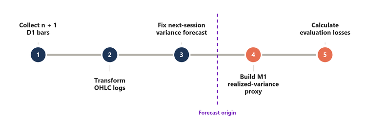
Image 1: Chronological separation between the completed D1 estimation window, fixed variance forecast, next-session M1 realized-variance proxy, and calculation of the evaluation losses.

QLIKE requires positive operands. The script applies the same lower bound of 1e-12 separately to a variance forecast and to a realized-variance proxy only when that operand is at or below the bound. It counts every floor event. The reported comparison contained zero floor events, so its QLIKE values come directly from the forecasts and proxies.

MQL5 module architecture

HistoricalVolatilityEstimators.mqh contains no global input dependency. Configuration enters through method parameters or SetNegativeTolerance(). Every class method is declared in the class interface and implemented externally with CHistoricalVolatilityEstimators::MethodName.

Public data contract

The enum fixes the estimator order used by the include module, indicator, comparison script, CSV rows, and result tables. SVarianceEstimates keeps the five historical variance estimates together, while SRealizedVarianceDetails stores the realized-variance proxy components and M1 diagnostics. The class exposes calculation and selection through method parameters and does not read host inputs.

Component	Responsibility
ENUM_HISTORICAL_VARIANCE_ESTIMATOR	Stable dispatch for the five estimator names and values.
SVarianceEstimates	Five variance estimates from one estimation window, Yang-Zhang coefficient, validity, and exact error.
SRealizedVarianceDetails	Close-to-open jump, intraday and total realized-variance proxy, M1 coverage, gap diagnostics, and status.
CalculateAll()	Validates one chronological n + 1 D1 estimation window, transforms log terms once, and calculates all five variances.
CalculateRealizedVariance()	Validates the interval of one forecast target and aggregates the close-to-open jump exactly once plus M1 squared returns.
CompareVolatilityEstimators.mq5	Loads history, applies the chronological loop and common target mask, scores retained forecast targets, prints summaries, and exports CSV evidence.
AnalyzeVolatilityEstimatorRobustness.mq5	Calculates paired circular moving-block bootstrap intervals and the past-only rolling scale calibration from the detailed observations.

CopyRates() places the oldest copied element at the start of physical memory regardless of the target array’s series flag. The scripts still call ArraySetAsSeries() explicitly with the series flag set to false. The include module rejects non-increasing timestamps, causing a reversed array to fail validation instead of altering the chronological input.

Every OHLC tuple must be finite and positive. High cannot be below open, close, or low; low cannot exceed them. The estimation window must contain at least two return intervals, and the array size must be exactly n + 1. These guards run before any logarithm.

The comparison script writes detailed observations, a summary, and a session-audit CSV. The audit records one status per candidate session. The robustness script reads the detailed observations and writes the paired circular moving-block bootstrap and past-only rolling scale calibration CSV files.

Chronological scoring and export

After both the calculation for the common estimation window and forecast target are valid, the script calculates all three evaluation losses from non-annualized variance. Only the two QLIKE operands receive the declared positive floor; MAE and RMSE use the unmodified variance forecast and realized-variance proxy. Each accepted observation is then written to the detailed CSV and passed to the corresponding estimator accumulator for that estimation window.

Deterministic validation

Estimator calculations require tests that are independent of broker history. A fixed OHLC sequence provides exact expected values for detecting denominator errors, shifted previous closes, an incorrect Yang-Zhang coefficient, or sign errors in the Rogers-Satchell terms.

A flat sequence should return zero. Multiplying all prices by one positive constant should leave log-return variance unchanged. Reversed timestamps should be rejected, and an invalid estimator enum should fail without publishing a value. A fixed M1 fixture can also confirm that the close-to-open jump is included exactly once.

ValidateVolatilityEstimators.mq5 implements 23 deterministic checks. Its target-mutation check changes only future-target prices while leaving the array supplied to CalculateAll() untouched, then verifies identical estimator outputs. This confirms the local CalculateAll() invariant; it does not by itself prove the absence of look-ahead in the complete history-loading and scoring pipeline. The separate timestamp and interval checks address that broader workflow.

Using the attached indicator

HistoricalVolatilityEstimatorIndicator.mq5 turns the same include module into a separate-window indicator. It can display all five lines or one selected estimator and supports changes to the estimation window and output unit.

Only a D1 chart reproduces the daily inputs and interpretation of this study. On any other timeframe, the indicator estimates variance per active chart bar and is not directly comparable with the D1 study results. Annualization is optional and disabled by default. InpCompletedBarsOnly=true leaves the current bar empty.

The default display is non-annualized per-bar volatility, obtained as the square root of the per-bar variance; on D1, this is daily volatility. This affects only the plotted unit, while the comparison tables and evaluation losses remain in non-annualized daily variance. Selecting the annualization option multiplies variance by InpPeriodsPerYear before applying the square root when volatility is displayed.

The three local helpers below define the display conversion, complete MqlRates reconstruction, and synchronized empty-buffer behavior used by OnCalculate().

//+------------------------------------------------------------------+
//| Convert raw per-bar variance to the selected display unit        |
//+------------------------------------------------------------------+
double DisplayValue(const double variance)
  {
//--- Start from the validated nonannualized per-bar variance.
   double value=variance;
//--- Apply the configured periods-per-year factor before conversion.
   if(InpAnnualize)
      value*=InpPeriodsPerYear;
//--- Convert variance to volatility only when the display requests it.
   if(InpDisplay==DISPLAY_VOLATILITY)
      value=::MathSqrt(value);
//--- Return one value in the unit named by the indicator short name.
   return(value);
  }

//+------------------------------------------------------------------+
//| Copy one OnCalculate price tuple into one complete MqlRates bar  |
//+------------------------------------------------------------------+
void SetRate(MqlRates &bar,
             const int source,
             const datetime &time[],
             const double &open[],
             const double &high[],
             const double &low[],
             const double &close[],
             const long &tick_volume[],
             const long &volume[],
             const int &spread[])
  {
//--- Copy every source field used by validation or estimator output.
   bar.time=time[source];
   bar.open=open[source];
   bar.high=high[source];
   bar.low=low[source];
   bar.close=close[source];
   bar.tick_volume=tick_volume[source];
   bar.spread=spread[source];
   bar.real_volume=volume[source];
  }

//+------------------------------------------------------------------+
//| Reset every output buffer at one series shift                    |
//+------------------------------------------------------------------+
void SetEmpty(const int shift)
  {
//--- Keep all plots synchronized when one window cannot be calculated.
   g_close_to_close[shift]=EMPTY_VALUE;
   g_parkinson[shift]=EMPTY_VALUE;
   g_garman_klass[shift]=EMPTY_VALUE;
   g_rogers_satchell[shift]=EMPTY_VALUE;
   g_yang_zhang[shift]=EMPTY_VALUE;
  }

The following block contains the complete OnCalculate() implementation reproduced from the styled attachment without omission. The function normalizes input arrays, rejects insufficient histories, handles terminal-requested history resets, reconstructs each estimation window of n + 1 bars in chronological order, and publishes all five buffers from the common calculation.

//+------------------------------------------------------------------+
//| Calculate the selected estimator lines                           |
//+------------------------------------------------------------------+
int OnCalculate(const int rates_total,
                const int prev_calculated,
                const datetime &time[],
                const double &open[],
                const double &high[],
                const double &low[],
                const double &close[],
                const long &tick_volume[],
                const long &volume[],
                const int &spread[])
  {
//--- Normalize every OnCalculate input to current-bar-first indexing.
   ::ArraySetAsSeries(time,true);
   ::ArraySetAsSeries(open,true);
   ::ArraySetAsSeries(high,true);
   ::ArraySetAsSeries(low,true);
   ::ArraySetAsSeries(close,true);
   ::ArraySetAsSeries(tick_volume,true);
   ::ArraySetAsSeries(volume,true);
   ::ArraySetAsSeries(spread,true);

//--- Require n+1 available bars before calculating the oldest value.
   const int maximum_shift=rates_total-InpWindow-1;
   if(maximum_shift<0)
      return(0);

//--- Reinitialize after first attachment, history reset, or invalid state.
   const bool full_reset=(prev_calculated<=0 ||
                          prev_calculated>rates_total);
   if(full_reset)
     {
      ::ArrayInitialize(g_close_to_close,EMPTY_VALUE);
      ::ArrayInitialize(g_parkinson,EMPTY_VALUE);
      ::ArrayInitialize(g_garman_klass,EMPTY_VALUE);
      ::ArrayInitialize(g_rogers_satchell,EMPTY_VALUE);
      ::ArrayInitialize(g_yang_zhang,EMPTY_VALUE);
     }

//--- Recalculate all bars initially and only affected bars thereafter.
   int limit=maximum_shift;
   if(!full_reset)
      limit=::MathMin(maximum_shift,rates_total-prev_calculated+1);

//--- Keep the current bar empty when completed-window output is required.
   const int minimum_shift=(InpCompletedBarsOnly ? 1 : 0);
   if(InpCompletedBarsOnly)
      SetEmpty(0);

//--- Allocate one reusable chronological n+1-bar calculation window.
   MqlRates window_rates[];
   ::ArrayResize(window_rates,InpWindow+1);
   ::ArraySetAsSeries(window_rates,false);

//--- Process affected chart shifts from the oldest toward the newest.
   for(int shift=limit;shift>=minimum_shift;shift--)
     {
      //--- Reverse series indexes into physical oldest-to-newest order.
      for(int position=0;position<=InpWindow;position++)
        {
         const int source=shift+InpWindow-position;
         SetRate(window_rates[position],
                 source,
                 time,
                 open,
                 high,
                 low,
                 close,
                 tick_volume,
                 volume,
                 spread);
        }

      //--- Reject the complete plot row when common-window validation fails.
      SVarianceEstimates estimates;
      if(!g_calculator.CalculateAll(window_rates,InpWindow,estimates))
        {
         SetEmpty(shift);
         continue;
        }

      //--- Convert and publish every valid estimator in the selected unit.
      g_close_to_close[shift]=DisplayValue(estimates.close_to_close);
      g_parkinson[shift]=DisplayValue(estimates.parkinson);
      g_garman_klass[shift]=DisplayValue(estimates.garman_klass);
      g_rogers_satchell[shift]=DisplayValue(estimates.rogers_satchell);
      g_yang_zhang[shift]=DisplayValue(estimates.yang_zhang);
     }

//--- Report that every available input bar has been processed.
   return(rates_total);
  }

The resulting D1 indicator view is shown below.

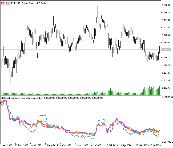
Image 2: HistoricalVolatilityEstimatorIndicator.mq5 attached to a D1 chart.

MetaTrader sets prev_calculated to zero when deeper history is loaded or history gaps are filled, as specified in the official OnCalculate() reference. Input changes cause deinitialization and reinitialization, as specified in the official OnDeinit() reference.

The implementation therefore treats prev_calculated <= 0 or the defensive case prev_calculated > rates_total as a full reset. Other calls recalculate only affected shifts, and a failed window empties all five buffers at that shift. These terminal-state safeguards do not enter the forecast comparison.

Integration steps

The package supports four operational paths. Readers can run the attached indicator, call the shared include module, execute the comparison script, or run the robustness script on the exported observations.

Running the attached indicator

The operating sequence is:

1. Compile HistoricalVolatilityEstimatorIndicator.mq5 in MQL5\Indicators\VolatilityEstimatorStudy and attach it to a chart from the Navigator.
2. Use a D1 chart to reproduce the daily interpretation used in this study; on another timeframe, each estimate is expressed per chart bar.
3. Set InpWindow to the required number of return intervals. Use 20 for the main study configuration.
4. Use InpDisplay to select variance or volatility and InpPlots to display all five estimators or one selected estimator.
5. Keep InpAnnualize=false and InpCompletedBarsOnly=true for the non-annualized completed-bar view used here. InpPeriodsPerYear is applied only when annualization is enabled.

Calling the include module

The include module needs a chronological n + 1 D1 array. After history has been loaded and validated, the surrounding program creates the calculator, sets its numerical tolerance, calls CalculateAll(), and selects the required output through SelectEstimate().

The module-integration sequence is:

1. Copy completed D1 history and normalize it to chronological physical order.
2. Create exactly n + 1 bars ending at the forecast origin.
3. Call CalculateAll() once and select each estimator output.
4. After the session of the forecast target exists, slice its M1 bars to the D1 boundaries and call CalculateRealizedVariance().
5. Score only when both the calculation for the common estimation window and forecast target are valid.

Reproducing the study and generating the CSV files

CompareVolatilityEstimators.mq5 is a standalone script. It loads the requested D1 and M1 history, applies fixed windows of 10, 20, and 40 sessions, constructs the common target mask, and writes the detailed, summary, and session-audit CSV files. AnalyzeVolatilityEstimatorRobustness.mq5 then reads the detailed observations for n=20.

To reproduce the reported study:

1. Place the include module and all three scripts in the terminal-relative locations shown in the file manifest, then compile them in MetaEditor.
2. In MetaTrader, confirm that the exact broker symbol is available and that its D1 and M1 history can be synchronized. Run CompareVolatilityEstimators.mq5 from the Scripts section of the Navigator. InpSymbolName, rather than the chart symbol, selects the instrument.
3. For the reported run, use the MetaQuotes-Demo environment with InpSymbolName=EURUSD, InpTargetStart=D'2020.01.01 00:00', and InpTargetEnd=D'2025.12.31 23:59'.
4. Keep the data-quality inputs at InpMinimumM1Bars=1380, InpMaximumM1Gap=300 seconds, and InpEndpointTolerance=1e-10. Keep InpQlikeFloor=1e-12 and InpHistoryRetries=3.
5. Confirm that the Experts log reports PASS and that 1,472 sessions are valid. The script writes volatility_estimator_observations.csv, volatility_estimator_summary.csv, and volatility_estimator_session_audit.csv.
6. Run AnalyzeVolatilityEstimatorRobustness.mq5 with a 252-session past-only rolling scale calibration window, 20-session blocks for the paired circular moving-block bootstrap, 10,000 replications, and seed 260924. Confirm PASS and preserve its two output CSV files.

Each script opens its outputs with FILE_WRITE: the comparison script recreates three CSV files, and the robustness script recreates two. Preserve an earlier export before repeating the study. To apply the same workflow to another instrument, set InpSymbolName to its exact broker symbol and set InpTargetStart and InpTargetEnd to the required target dates. The resulting valid-session count, losses, and rankings are specific to that symbol, quote history, broker-session convention, and period.

The main empirical results produced by this workflow are presented next.

Main empirical comparison

The declared primary criterion is mean QLIKE at n=20. MAE and RMSE evaluate error magnitude in daily-variance units; the bias ratio and correlation provide mean-scale and co-movement diagnostics. The paired circular moving-block bootstrap evaluates the Parkinson–Yang-Zhang evaluation-loss difference rather than treating a small rank difference as evidence of superiority.

Estimator	N	MAE	RMSE	Mean QLIKE	Bias ratio	Correlation	MAE rank	RMSE rank	QLIKE rank
Close-to-Close	1,472	1.1803472e-05	2.3576311e-05	0.20532776	0.863071	0.504389	5	5	5
Parkinson	1,472	1.0667907e-05	2.2742925e-05	0.15741134	0.883900	0.538499	1	2	1
Garman-Klass	1,472	1.0725768e-05	2.2692899e-05	0.15879607	0.895270	0.540816	2	1	3
Rogers-Satchell	1,472	1.0912125e-05	2.2892759e-05	0.16802282	0.892602	0.533854	4	4	4
Yang-Zhang	1,472	1.0875694e-05	2.2803784e-05	0.15808552	0.908638	0.537615	3	3	2

Parkinson had the lowest raw mean QLIKE and MAE at n=20. Garman-Klass had the lowest RMSE and highest correlation, while Yang-Zhang had the bias ratio closest to one. No estimator ranked first across all reported diagnostics.

Parkinson’s raw mean QLIKE was 0.00067418, or 0.426%, below Yang-Zhang. The 95% interval from the paired circular moving-block bootstrap for the session-level Parkinson–Yang-Zhang difference was [−0.00678547, 0.00507249]. Because the interval includes zero, this run does not distinguish the two estimators statistically under raw QLIKE.

The OHLC estimators all had lower raw MAE, RMSE, and QLIKE than Close-to-Close in this sample. This ordering does not isolate a causal benefit from the D1 high–low range: the formulas differ in their assumptions and transformations, and the M1 realized-variance proxy does not observe every D1 range excursion.

The main QLIKE values are shown on their own axis; no unit from another evaluation loss is mixed into the chart.

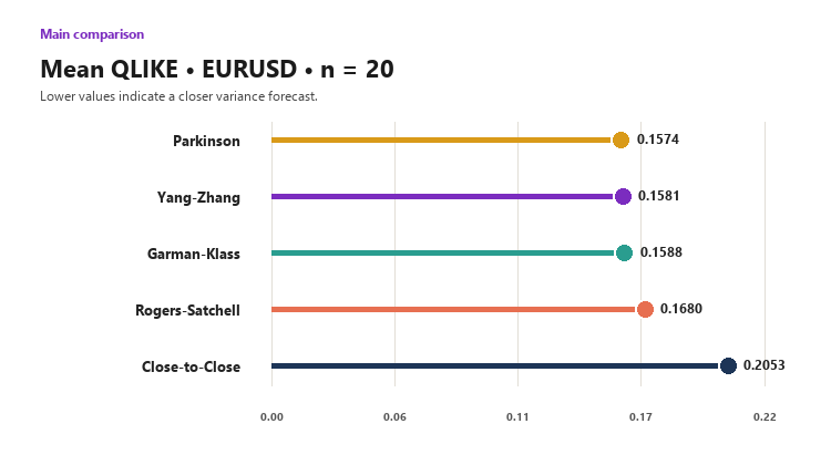
Image 3: Sorted raw mean QLIKE for 1,472 EURUSD forecast targets retained by the common target mask from 2020 through 2025 under the 20-session estimation window.

Ranks permit the three evaluation losses to be compared without placing MAE, RMSE, and QLIKE on one numeric scale.

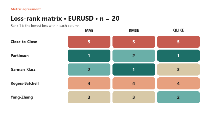
Image 4: Rank heatmap for MAE, RMSE, and QLIKE in the main EURUSD estimation window; rank 1 denotes the lowest evaluation loss.

Every bias ratio remained below one. Yang-Zhang had the closest average scale agreement, while Garman-Klass produced the highest correlation and lowest RMSE. Neither diagnostic replaced QLIKE: average scale agreement can coexist with offsetting session-level errors, and correlation does not measure the forecast level. Because these rankings use n=20, sensitivity to the estimation window is checked separately.

Past-only rolling scale calibration

For each eligible target, the past-only rolling scale calibration multiplies the raw forecast by mean(RV / h) calculated from only the preceding 252 valid sessions for that estimator. The first 252 observations initialize the scale factor and are not scored, leaving 1,220 calibrated forecasts. No future target enters a scale factor.

Estimator	Calibrated QLIKE	Rank
Close-to-Close	0.16917167	5
Parkinson	0.13138316	3
Garman-Klass	0.13106313	2
Rogers-Satchell	0.13399977	4
Yang-Zhang	0.13052278	1

After the past-only rolling scale calibration, Yang-Zhang had the lowest mean QLIKE and Parkinson ranked third. The calibrated Parkinson–Yang-Zhang difference was 0.00086038, with a 95% interval from the paired circular moving-block bootstrap of [−0.00434904, 0.00595155]. The interval again includes zero. The reversal of the point ranking shows that the raw order is scale-sensitive; neither version supports a claim that Parkinson is substantively superior to Yang-Zhang.

Sensitivity to the estimation window

The sensitivity analysis keeps every other convention fixed. Garman-Klass had the lowest raw QLIKE at n=10, while Parkinson had the lowest at n=20 and n=40. The RMSE leader was Garman-Klass at n=10 and n=20, then Parkinson at n=40. The ranking is therefore sensitive to both the window and the loss.

Estimator	QLIKE n=10	Rank	QLIKE n=20	Rank	QLIKE n=40	Rank
Close-to-Close	0.31079548	5	0.20532776	5	0.18777780	4
Parkinson	0.14836057	3	0.15741134	1	0.17825365	1
Garman-Klass	0.14398123	1	0.15879607	3	0.18054721	3
Rogers-Satchell	0.15352112	4	0.16802282	4	0.18858413	5
Yang-Zhang	0.14418616	2	0.15808552	2	0.18025839	2

Changing n changes the balance between responsiveness and smoothing. A shorter estimation window assigns greater relative influence to each observation and responds sooner to changes in recent ranges. A longer window distributes influence across more observations and changes more gradually. The selected length therefore depends on the required balance between adaptation speed and estimate stability; it should not be chosen solely from the minimum evaluation loss in one sample.

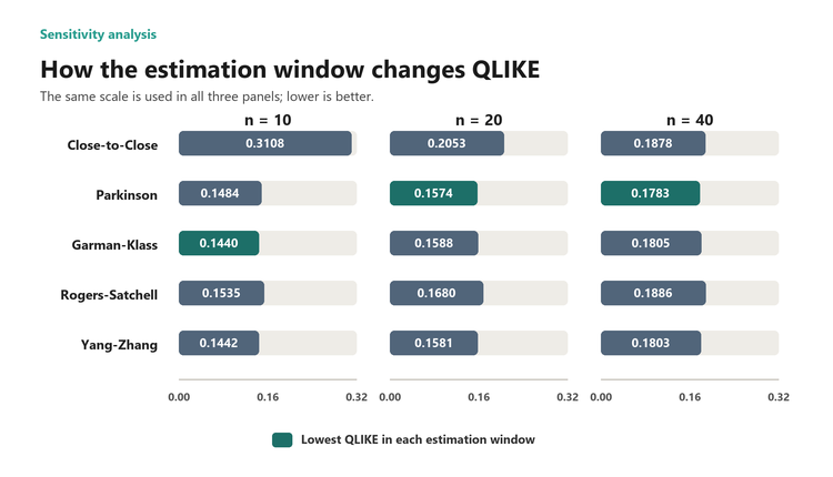
Image 5: Shared-scale comparison of mean QLIKE under the three EURUSD estimation windows; the lowest value in each panel is highlighted.

Close-to-Close improved as n increased, while the four OHLC estimators had their lowest raw QLIKE at n=10. Garman-Klass led at n=10; Parkinson led at n=20 and n=40. Yang-Zhang ranked second in all three windows. The estimation window must therefore be reported as part of the model specification.

Yang-Zhang explicitly represents close-to-open movement, but this feature did not give it the lowest raw QLIKE in these windows. Estimator structure alone does not determine the ranking.

Limitations and safeguards

The reported results and attached implementation are subject to the following limitations and safeguards:

• Single environment: the findings describe EURUSD in the MetaQuotes-Demo history from 2020 through 2025. They do not establish ranking stability across symbols, brokers, quote sources, D1 boundaries, or periods.
• Proxy construction: forecasts use D1 OHLC data, while the target uses M1 closes and the close-to-open jump. The target can miss intraminute range excursions and is not latent integrated variance.
• Session construction: a broker D1 bar is not assumed to be an official exchange session. The 00:00 boundary and observed gaps belong to this server-time history.
• Persistence forecast: carrying the estimate forward isolates differences among estimators. It is not an optimized forecasting system and does not exploit additional predictors or fitted dynamics.
• Paired uncertainty: the paired circular moving-block bootstrap uses 20-session blocks to preserve short-range evaluation-loss dependence. The block length remains a modeling choice.
• Selection: the common target mask makes estimator samples identical but cannot remove selection induced by data availability, coverage thresholds, instrument choice, or the tested period.
• Variance units: every score uses non-annualized daily variance. Annualized volatility is not inserted into any column for an evaluation loss, so variance, volatility, and standard deviation are never mixed.
• No trading conclusion: the scripts do not test entries, exits, spread, slippage, commission, execution, position sizing, or profitability. A lower evaluation loss does not imply a profitable trade.

Conclusion

The include module, scripts, indicator, and CSV files provide an auditable pipeline. It maps broker OHLC history to:

• five variance estimates from a common window,
• one-session-ahead persistence forecasts,
• an M1 realized-variance proxy,
• documented exclusions and evaluation summaries.

MQL5 developers can change the estimator without changing the estimation windows, common target mask, or definitions of the evaluation losses.

For the raw EURUSD comparison at n=20, Parkinson had the lowest mean QLIKE and MAE across 1,472 retained targets. Garman-Klass had the lowest RMSE and highest correlation, while Yang-Zhang had the bias ratio closest to one. The raw QLIKE leader changed from Garman-Klass at n=10 to Parkinson at n=20 and n=40.

The raw Parkinson–Yang-Zhang difference was small, and its 95% interval from the paired circular moving-block bootstrap included zero. Under the past-only rolling scale calibration, Yang-Zhang had the lowest point QLIKE, but its corresponding interval also included zero. The defensible conclusion is therefore a reproducible, window- and scale-sensitive comparison for one MetaQuotes-Demo EURUSD sample, not a generally superior estimator.

Primary references

• Michael Parkinson, “The Extreme Value Method for Estimating the Variance of the Rate of Return,” The Journal of Business 53(1), 1980, DOI 10.1086/296071.
• Mark B. Garman and Michael J. Klass, “On the Estimation of Security Price Volatilities from Historical Data,” The Journal of Business 53(1), 1980, DOI 10.1086/296072.
• L. C. G. Rogers and S. E. Satchell, “Estimating Variance From High, Low and Closing Prices,” The Annals of Applied Probability 1(4), 1991, DOI 10.1214/aoap/1177005835.
• Dennis Yang and Qiang Zhang, “Drift-Independent Volatility Estimation Based on High, Low, Open, and Close Prices,” The Journal of Business 73(3), 2000, DOI 10.1086/209650.
• Andrew J. Patton, “Volatility Forecast Comparison Using Imperfect Volatility Proxies,” Journal of Econometrics 160(1), 2011, DOI 10.1016/j.jeconom.2010.03.034.
• Hans R. Künsch, “The Jackknife and the Bootstrap for General Stationary Observations,” The Annals of Statistics 17(3), 1989, DOI 10.1214/aos/1176347265.

File manifest

File name	Description
MQL5\Include\VolatilityEstimatorStudy\HistoricalVolatilityEstimators.mqh	Reusable five-estimator variance and realized-variance proxy calculations.
MQL5\Indicators\VolatilityEstimatorStudy\HistoricalVolatilityEstimatorIndicator.mq5	Configurable separate-window display for one or all five estimators.
MQL5\Scripts\VolatilityEstimatorStudy\CompareVolatilityEstimators.mq5	Chronological EURUSD comparison, metrics, diagnostics, terminal summary, and CSV export.
MQL5\Scripts\VolatilityEstimatorStudy\ValidateVolatilityEstimators.mq5	Deterministic formula, guard, aggregation, order, scale, and no-lookahead tests.
MQL5\Scripts\VolatilityEstimatorStudy\AnalyzeVolatilityEstimatorRobustness.mq5	Paired circular moving-block bootstrap and past-only rolling scale calibration analysis for the main window.
MQL5\Files\VolatilityEstimatorStudy\Examples\volatility_estimator_observations.csv	Detailed 2020–2025 variance forecasts, realized-variance proxies, evaluation losses, and M1 coverage evidence.
MQL5\Files\VolatilityEstimatorStudy\Examples\volatility_estimator_summary.csv	Final estimator metrics and descriptive ranks for each estimation window.
MQL5\Files\VolatilityEstimatorStudy\Examples\volatility_estimator_session_audit.csv	One status row for each of the 1,560 candidate broker D1 sessions.
MQL5\Files\VolatilityEstimatorStudy\Examples\volatility_estimator_robustness.csv	Raw and calibrated Parkinson–Yang-Zhang differences with paired circular moving-block bootstrap intervals.
MQL5\Files\VolatilityEstimatorStudy\Examples\volatility_estimator_calibrated_summary.csv	Past-only rolling scale calibration QLIKE values and ranks at n=20.