

MetaTrader 5機械学習の設計図(第7回):散発的な実験から再現可能な結果へ
 136
136
 0
0

はじめに
本連載では、機械学習をトレードへ応用するための重要な要素として、データ構造、ラベリングおよびメタラベリング、サンプル重み付け、そしてPurged Cross-Validation(パージド交差検証)を取り上げてきました。しかし、これらの手法は個別でも強力である一方、その真価を発揮するのは、一貫したリサーチシステムへ統合されたときです。本記事では、これらの構成要素をどのように組み合わせ、場当たり的な実験を再現可能かつ監査可能なリサーチプロセスへと変え、さらに前回の記事で構築したキャッシュアーキテクチャを土台として、本番運用レベルのパイプラインを組み上げる方法を紹介します。
これから見ていくコードは、よくあるサンプルコードではなく、私が実際にトレードモデルを開発する際に使っているシステムの重要な一部です。このシステムは、生のティックデータから、MetaTrader 5で利用可能なONNXモデルの生成までを一貫して処理し、その過程で包括的なログ、キャッシュ、分析レポートを自動的に生成します。なお、説明を分かりやすくするため、本記事では特徴量重要度の分析や、トリプルバリア法における最適なバリア設定の選択といった重要なテーマについてはここではいったん割愛します。これらのリサーチステップはすでに完了していることを前提とし、本記事では再現性のあるパイプラインの構築に焦点を当てます。リサーチシステムが「本番運用レベル」であるとは、どういうことでしょうか。
- 再現性:同じコードを何度実行しても、常に同じ結果が得られること。
- トレーサビリティ:各モデルがどのデータを用いて学習されたのかを正確に把握できること。
- 効率性:計算コストの高い処理をキャッシュし、不要な再計算をしないこと。
- 検証:問題を本番環境へ持ち込む前に検出できること。
- ドキュメント:意思決定の根拠を説明するレポートを自動生成できること。
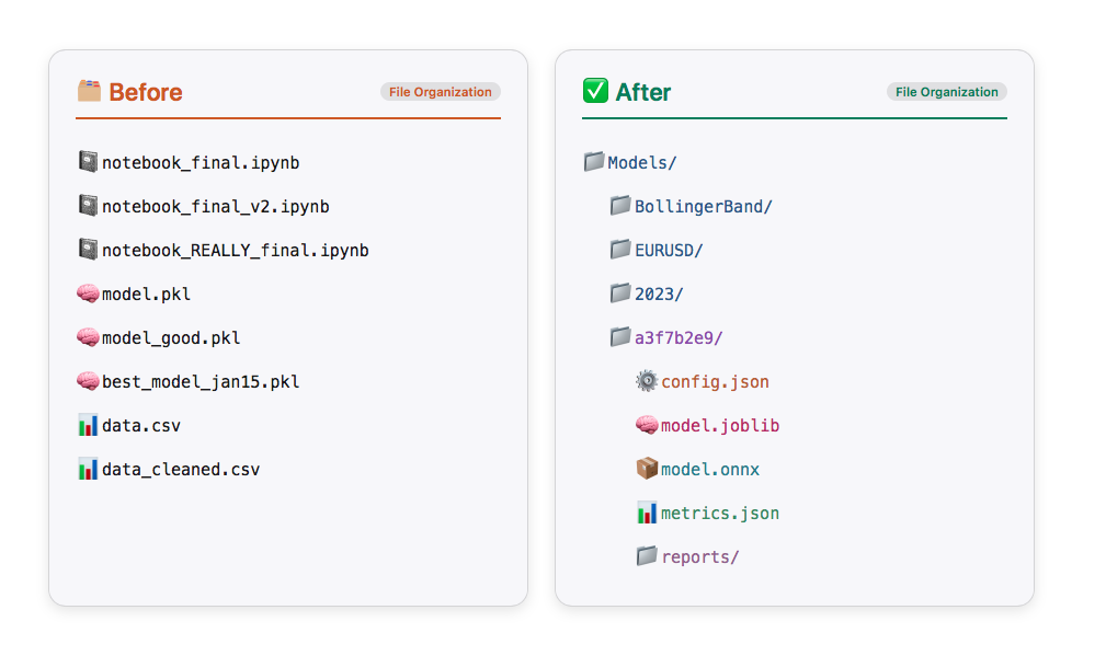
問題点:リサーチの混沌
解決策に入る前に、まず現状の問題を確認しましょう。多くの機械学習を用いたトレードリサーチは、次のような状態になっています。
# Somewhere in notebook cell 47...

df = load_data("EURUSD", "2020-01-01", "2023-12-31")
features = calculate_indicators(df)
X_train, y_train = features[:-1000], labels[:-1000]
model = RandomForestClassifier(n_estimators=100)
model.fit(X_train, y_train)

# Score: 0.67 - is that good? What parameters did I use?
# When did I run this? Which data version?
3か月後には、これらの結果を再現できなくなっています。データは更新され、どの特徴量を使用したのかも覚えていません。モデルファイルにはメタデータが含まれておらず、結局は振り出しに戻ってしまいます。
これは単に不便なだけではなく、非常に危険です。本番環境でのトレードにおいて、再現性のないリサーチはバックテストを信頼できないことを意味します。障害が発生しても原因を特定できず、安心して改善を重ねることもできません。
解決策:原則に基づいたパイプライン
本リサーチシステムでは、以下の4つの基本原則によってこれらの問題を解決します。
- 時間を考慮したキャッシュ:将来のデータが学習に混入しないようにしながら、安全にあらゆる計算結果をキャッシュします。
- 自動ドキュメント化:各段階で包括的なレポートを自動生成します。
- 整理されたストレージ:戦略、銘柄、パラメータごとに実験をたどれるように整理します。
- 検証優先:本番環境ではなく、リサーチ段階で問題を検出します。
システム全体のアーキテクチャは次のようになります。
すべての処理段階がキャッシュされ、すべての意思決定が記録され、すべての出力が検証されます。
ここで改めて強調しておきますが、これはあくまで高レベルなアーキテクチャであり、モデル開発プロセスのすべての工程を網羅することを目的としたものではありません。
インテリジェントなデータアーキテクチャ:ティックデータのRAMキャッシュとParquetバーがもたらすメリット
各パイプラインの詳細に入る前に、このシステム全体を実用的なものにしている重要な設計判断、すなわちデータ処理戦略について説明します。
ティックデータ処理における課題
トレード戦略を開発する際には、次のような典型的な選択を迫られます。
| オプション1:ブローカー(MetaTrader 5)から直接バーを読み込む | オプション2:すべてをディスクにキャッシュする | オプション3:ハイブリッド方式(推奨) |
|---|---|---|
|
|
|
この3番目の方法が優れている理由を見ていきましょう。
TickDataLoader:RAMキャッシュを活用した効率的なデータ管理
重要なポイントは、ティックデータはディスクではなくRAM上に保持すべきだということです。ティックデータは、さまざまな方法で加工・変換される元データだからです。TickDataLoaderクラスは、現在のセッション中に読み込んだすべてのデータを管理します。たとえば、最初に2023年のEURUSDデータを読み込み、その後2021~2022年のデータを追加することにした場合、既にキャッシュされているデータを再読み込みすることはありません。不足している期間のデータだけを取得し、既存のキャッシュへシームレスに追加します。つまり、TickDataLoaderはキャッシュに存在しないデータだけを取得し、それを事前に読み込まれているデータへ追記します。以下のコードはTickDataLoaderクラスからの抜粋です。完全なコードについては、添付のmodel_development.pyを参照してください。
class TickDataLoader:
    """
    Loader for tick-level bid/ask data with intelligent local caching.

    Features:
    1. Smart caching that checks if requested date range is within cached ranges
    2. Handles partial overlaps by reusing available cached data
    3. Memory management with cache size limits
    4. Cache statistics tracking

    Notes
    -----
    - Typical performance: ~0.5s for cached retrieval
    - Memory usage: ~100MB per 1M ticks
    """

    def __init__(self, max_cache_size_mb: int = 3000, max_cached_symbols: int = 20):
        """
        Initialize the tick data loader.

        Parameters
        ----------
        max_cache_size_mb : int, optional
            Maximum cache size in MB (default: 5000MB)
        max_cached_symbols : int, optional
            Maximum number of symbols to keep in cache (default: 20)
        """
        self._cache: Dict[Tuple[str, str], pd.DataFrame] = {}  # (symbol, account_name) -> DataFrame
        self._cache_metadata: Dict[Tuple[str, str], Dict] = {}  # (symbol, account_name) -> metadata
        self.max_cache_size_mb = max_cache_size_mb
        self.max_cached_symbols = max_cached_symbols
        self.cache_stats = {
            "hits": 0,
            "misses": 0,
            "partial_hits": 0,
            "total_loaded": 0,
        }

    def get_tick_data(
        self, symbol: str, start_date: str, end_date: str, account_name: str
    ) -> pd.DataFrame:
        """
        Retrieve tick-level bid/ask data with intelligent caching.

        Parameters
        ----------
        symbol : str
            Trading instrument symbol (e.g., 'EURUSD')
        start_date : str
            Start date in 'YYYY-MM-DD' format
        end_date : str
            End date in 'YYYY-MM-DD' format
        account_name : str
            MT5 account identifier for data retrieval

        Returns
        -------
        pd.DataFrame
            Tick data with columns ['bid', 'ask'] indexed by timestamp

        Notes
        -----
        - Checks if cached data fully covers requested date range
        - If partial coverage exists, loads only missing data
        - Merges cached and newly loaded data seamlessly
        """
        cache_key = (symbol, account_name)
        start_dt, end_dt = date_conversion(start_date, end_date)

        # Check if we have cached data for this symbol/account
        if cache_key in self._cache:
            cached_df = self._cache[cache_key]
            metadata = self._cache_metadata[cache_key]
            cached_start, cached_end = date_conversion(metadata["start_date"], metadata["end_date"])

            # Check if cached data fully covers requested range
            if cached_start <= start_dt and cached_end >= end_dt:
                self.cache_stats["hits"] += 1
                logger.debug(f"Cache hit for {symbol} {start_date} to {end_date}")

                # Return subset of cached data
                mask = (cached_df.index >= start_dt) & (cached_df.index <= end_dt)
                return cached_df[mask].copy()

            # Check if there's partial overlap
            if cached_end >= start_dt and cached_start <= end_dt:
                self.cache_stats["partial_hits"] += 1
                logger.debug(f"Partial cache hit for {symbol}")
                return self._load_with_partial_cache(
                    symbol, start_date, end_date, account_name, cache_key
                )

        # No cache hit, load all data
        self.cache_stats["misses"] += 1
        logger.debug(f"Cache miss for {symbol} {start_date} to {end_date}")
        return self._load_and_cache_data(symbol, start_date, end_date, account_name, cache_key)
このシステムは、以下の3つのシナリオをインテリジェントに処理します。
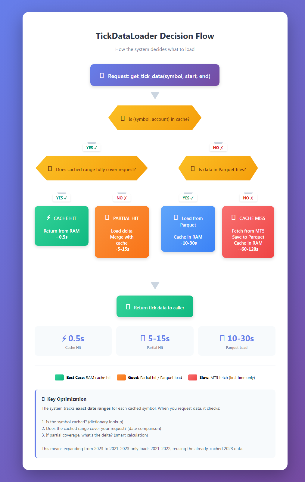
以下はTickDataLoaderクラスの使用例です。
# Initialize the loader once per session
from ..production.model_development import TickDataLoader

loader = TickDataLoader(
    max_cache_size_mb=3000, # 3GB RAM limit
    max_cached_symbols=20, # Cache up to 20 symbols
)

# First request - loads from disk/MT5 and caches
ticks = loader.get_tick_data(
    symbol="EURUSD",
    start_date="2023-01-01",
    end_date="2023-12-31",
    account_name="FUNDEDNEXT_STLR2_6K"
)
# Takes ~30 seconds (first load)

# Second request - same data, instant from RAM
ticks = loader.get_tick_data(
    symbol="EURUSD",
    start_date="2023-01-01",
    end_date="2023-12-31",
    account_name="FUNDEDNEXT_STLR2_6K"
)
# Takes ~0.5 seconds (cache hit)

# Partial request - subset is instant
ticks = loader.get_tick_data(
    symbol="EURUSD",
    start_date="2023-01-01",
    end_date="2023-03-31",
    account_name="FUNDEDNEXT_STLR2_6K"
)
# Takes ~0.5 seconds (subset from cache)

ticks = loader.get_tick_data(
    symbol="EURUSD",
    start_date="2022-01-01",
    end_date="2023-12-31",
    account_name="FUNDEDNEXT_STLR2_6K"
)
# Takes ~15 seconds (only 2022 data)
以下は、ティックデータを使用する機能です。
# Example of features that use tick data

from ..util.volatility import two_time_scale_realized_vol

def two_time_scale_realized_vol(
    tick_prices: pd.Series, slow_freq: str = "5min"
) -> float:
    """
    Two-Time-Scale Realized Volatility Estimator

    Advanced estimator for tick data that removes microstructure noise while
    preserving information. Combines high-frequency and low-frequency sampling
    to extract true volatility signal.

    **What it measures:**
    - True underlying volatility from noisy tick data
    - Removes bid-ask bounce and other microstructure effects
    - Preserves information lost in simple low-frequency sampling

    **Mathematical foundation:**
    - TSRV = RV_slow - (n_slow/n_fast) * (RV_fast - RV_slow)
    - Uses ratio of observation counts to properly scale noise estimate
    - Asymptotically consistent under jump-diffusion models

    **Best used for:**
    - High-frequency trading strategies
    - When you have access to tick data
    - Precision-critical applications (research, risk management)
    - Markets with significant microstructure noise

    **Advantages:**
    - Most accurate volatility estimate for tick data
    - Removes upward bias from microstructure noise
    - Retains more information than sparse sampling
    - Theoretically well-founded

    **Computational considerations:**
    - More intensive than simple realized volatility
    - Requires choice of slow sampling frequency
    - Benefits increase with data quality and frequency

    **Typical slow frequencies:**
    - 1 minute: Very liquid assets, high precision needed
    - 5 minutes: Most common, good noise reduction
    - 15-30 minutes: Less liquid assets

    :param tick_prices: (pd.Series) Tick-level price data, datetime indexed
    :param slow_freq: (str) Slow sampling frequency ('5min', '1min', etc.)
    :return: (float) Two-time-scale realized volatility estimate
    """
    # Fast scale (tick-by-tick)
    tick_returns = np.log(tick_prices / tick_prices.shift(1)).dropna()
    rv_fast = (tick_returns**2).sum()
    n_fast = len(tick_returns)

    # Slow scale (e.g., 5-minute)
    slow_prices = tick_prices.resample(slow_freq).last().dropna()
    slow_returns = np.log(slow_prices / slow_prices.shift(1)).dropna()
    rv_slow = (slow_returns**2).sum()
    n_slow = len(slow_returns)

    # Two-time-scale estimator with proper scaling
    if n_fast > 0 and n_slow > 0:
        tsrv = rv_slow - (n_slow / n_fast) * (rv_fast - rv_slow)
        return max(tsrv, 0)  # Ensure non-negative result
    else:
        return rv_slow


two_time_scale_vol = two_time_scale_realized_vol(tick_prices=ticks["bid"], slow_freq="5min")
なぜディスクではなくRAMなのか
普段おこなっているリサーチワークフローについて考えてみてください。
# You might experiment with:
tick_bars_M1 = make_bars(ticks, "tick", "M1", "mid_price")
tick_bars_M5 = make_bars(ticks, "tick", "M5", "mid_price")
volume_bars = make_bars(ticks, "volume", 1000, "mid_price")
dollar_bars = make_bars(ticks, "dollar", 5000, "mid_price")

# And different price types:
tick_bars_bid = make_bars(ticks, "tick", "M1", "bid")
tick_bars_ask = make_bars(ticks, "tick", "M1", "ask")
同じティックデータから6種類の異なるバーを作成するとします。もしティックデータもバーもディスクへキャッシュするのであれば、実質的には同じ元データを、少し集約方法を変えただけの形で何度も保存することになります。これはストレージの無駄です。さらに、後になってマイクロストラクチャ特徴量(ティックデータが必要な特徴量)を作成したくなるかもしれません。そのため、あとで必要になる可能性があるため、ティックデータはRAM上に保持しておくのが最適です。
そこで、本システムでは次のような方針を採用します。
- ティックデータはRAMに保持する(高速アクセス、セッション終了時に破棄)
- バーは設定ごとにParquet形式でキャッシュする(永続保存、省容量)
- ティックデータは、そのセッションにおける「唯一の信頼できる元データ(Source of Truth)」として扱う
- Parquetファイルは、長期保存のための「生成済みアーティファクト」として利用する
TickDataLoaderとParquetを組み合わせたアーキテクチャは、機械学習のリサーチにおける次の重要な原則に基づいています。
生データは高速に扱えるようRAMへ保持し、加工済みデータはParquetとして永続化する。そして、再生成できるデータは重複して保存しない。
このデータアーキテクチャは、個人でのリサーチからチーム開発まで自然に拡張できます。全員がParquetファイルを利用することで、次のようなメリットが得られます。
- データ型が常に統一される(「自分の環境では動くのに」という問題がなくなる)
- ストレージ効率が高く、バージョン管理にも適している
- 実験を高速に繰り返せる(実験コストがほぼゼロになる)
- Parquetファイルはバイナリレベルで安定しており、高い再現性を確保できる
これをCSVベースのワークフローと比較すると、CSVでは次のような問題に常に悩まされます。
- 日時フォーマットの解釈が環境によって異なる
- 浮動小数点数の精度の違い
- 文字コードの問題
- 読み込み速度が遅い
- ファイルサイズが大きい
- スキーマ検証が煩雑
Parquetベースのストレージ環境を最初に整備するためには多少の手間がかかります。しかし、その投資は日々のリサーチで大きな効果をもたらします。さらに、生データであるティックデータをRAM上でインテリジェントにキャッシュする仕組みと組み合わせることで、高速性と効率性を両立した、妥協のないシステムを実現できます。
ワークフロー
それでは、実際の例として、EURUSDのボリンジャーバンド逆張り戦略を開発する流れを見ていきましょう。各ステージで何がおこなわれ、どのような成果物(アーティファクト)が生成されるのかを順を追って説明します。
ステージ1:設定
すべては設定ファイルから始まります。複数のファイルにパラメータを分散させるのではなく、単一の情報源として一元管理された設定を用います。
from model_development import ModelDevelopmentPipeline
from strategies import BollingerBandStrategy

# Data configuration
data_config = {
    "symbol": "EURUSD",
    "train_start": "2023-01-01",
    "train_end": "2023-12-31",
    "account_name": "FUNDEDNEXT_STLR2_6K",
    "bar_type": "tick",
    "bar_size": "M1",  # Will be converted to tick count
    "price": "mid_price"
}

# Feature configuration
feature_config = {
    "func": calculate_bollinger_features,
    "params": {
        "window": 20,
        "num_std": 2.0
    }
}

# Triple-barrier labeling
target_config = {
    "func": get_daily_vol,
    "params": {"lookback": 20}
}

label_config = {
    "profit_target": 1.0,
    "stop_loss": 2.0,
    "max_holding_period": {"days": 1},
    "min_ret": 0.0,
    "vertical_barrier_zero": True,
    "filter_as_series": False
}

# Model training parameters
model_params = {
    "pipe_clf": RandomForestClassifier(
        criterion="entropy",
        class_weight="balanced_subsample",
        min_weight_fraction_leaf=0.05
    ),
    "param_grid": {
        "n_estimators": [100, 200, 300],
        "max_depth": [3, 5, 7, 10],
        "min_samples_split": [2, 5, 10]
    },
    "cv_splits": 5,
    "bagging_n_estimators": 10,
    "n_jobs": -1,
    "random_state": 42
}

# Initialize strategy
strategy = BollingerBandStrategy(
    window=20,
    std=2.0,
)
すべてのパラメータが明示され、文書化されていることに注目してください。3か月後でも、自分が何をしたのか正確にわかるでしょう。
ステージ2:パイプラインの初期化
それでは、インテリジェントなファイル管理機能を備えたパイプラインを作成します。
pipeline = ModelDevelopmentPipeline(
    strategy=strategy,
    data_config=data_config,
    feature_config=feature_config,
    target_config=target_config,
    label_config=label_config,
    model_params=model_params,
    base_dir="Models"
)
バックグラウンドでは、この処理によって次のような構造化されたディレクトリが自動的に作成されます。 Models/ └── BollingerBandStrategy/ └── EURUSD/ └── FUNDEDNEXT_STLR2_6K/ └── tick/ └── M1/ └── 20230101_20231231/ └── a3f7b2e9/ # Config hash ├── config.json ├── logs/ ├── plots/ └── reports/各設定にはそれぞれ専用のディレクトリが割り当てられます。「model_v2_final_REALLY_FINAL.pkl」はもう存在しません。
ステージ3:実行
設定が完了したら、パイプライン全体を実行します。
model, features, metrics, config = pipeline.run(
    generate_reports=True,
    save=True,
    export_onnx=True,
    verbose=True
)
ここから実際の処理が動き始めます。各段階での処理を見ていきましょう。
ステップ1:データ読み込み(スマートキャッシング機能付き)
[Step 1/7] Loading training data...
✓ Cache hit for EURUSD 2023-01-01 to 2023-12-31
✓ Retrieved 15,847,392 ticks in 0.4s
✓ Constructed 262,800 M1 bars
システムは、対象となるデータがすでに読み込まれているかどうかを確認します。すでに読み込まれている場合は、数分かかる再読み込みをおこなうのではなく、キャッシュから数ミリ秒で取得できます。しかし、ここで重要なのは、このキャッシュが時間を考慮した仕組みになっていることです。システムは「いつ」「どのデータにアクセスしたか」を記録しており、将来のデータが誤って学習データセットへ混入することを防ぎます。
# From model_development.py
@cacheable(time_aware=True)
def load_and_prepare_training_data(symbol, start_date, end_date, ...):
    tick_df = loader.get_tick_data(symbol, start_date, end_date, account_name)
    data = make_bars(tick_df, bar_type, bar_size, price)

    # Log data access for contamination tracking
    log_data_access(
        dataset_name=f"{symbol}_{bar_type}_{bar_size}_{price}".lower(),
        start_date=data.index[0],
        end_date=data.index[-1],
        purpose="train"
    )

    return data
ステップ2:特徴量エンジニアリング
✓ Generated 47 features
- 12 Bollinger Band features
- 15 momentum features
- 8 volume features
- 12 time-based features
@cacheable(time_aware=True)
def create_feature_engineering_pipeline(data, feature_config, data_config):
    func = feature_config["func"]
    features = func(data, **feature_config["params"])
    time_feat = get_time_features(data, timeframe=data_config["bar_size"])
    return features.join(time_feat).dropna()
特徴量関数が変更されると、キャッシュは自動的に無効化されます。データのみが変更された場合、特徴量は効率的に再計算されます。
ステップ3:ラベル生成
[Step 3/7] Generating events...
✓ Generated 89,247 events
✓ Label distribution:
- Long (1):38,562 (43.2%)
- None (0):24,891 (27.9%)
- Short (-1):25,794 (28.9%)
@cacheable()
def generate_events_triple_barrier(data, strategy, target_config,
                                   profit_target, stop_loss, ...):
    # Calculate dynamic barriers based on volatility
    close = data["close"]
    fn = target_config["func"]
    params = target_config["params"]
    target = fn(close, **params)

    # Get entry signals from strategy
    side, t_events = get_entries(strategy, data, target.mean())

    # Apply triple-barrier method
    vb = add_vertical_barrier(t_events, close, **max_holding_period)
    events = triple_barrier_labels(close, target, t_events,
                                   vertical_barrier_times=vb,
                                   side_prediction=side,
                                   pt_sl=[profit_target, stop_loss], ...)

    # Add sample weights
    events = get_event_weights(events, close)
    return events
ステップ4:サンプル重みの最適化
ここからが面白いところです。サンプルの重みを推測するのではなく、最適な重み付け方式を探索します。
Testing weighting schemes:
- unweighted + linear decay
- unweighted + exponential decay
- return-based + linear decay
- return-based + exponential decay
- uniqueness + linear decay
- uniqueness + exponential decay
✓ Best scheme: uniqueness_linear_0.7428 (CV Score:0.6847)
システムは複数の重み付け手法を試し、パージド交差検証で最も性能の良いものを選択します。
@cacheable()
def get_optimal_sample_weight(
    data_index: pd.DatetimeIndex,
    events: pd.DataFrame,
    features: pd.DataFrame,
    cv_splits: int = 5,
    n_iter: int = 10,
) -> pd.Series:
    """
    Compute best sample weight with time decay.

    Parameters
    ----------
    data_index: pd.DatetimeIndex
        Price data index.
    events : pd.DataFrame
        Event labels with uniqueness weights.
    features: pd.DataFrame
        Training features
    cv_splits : int, optional
        Number of cross-validation splits (default: 5).
    n_iter : int, optional
        Number of random search iterations (default: 10).

    Returns
    -------
    weights : pd.Series
        Computed sample weights.
    cv_results : dict
        Cross-validation results.
    """
    valid_index = features.index.intersection(events.index)
    cont = events.loc[valid_index]
    X = features.loc[valid_index]
    y = cont["bin"]

    classifier = RandomForestClassifier(
        criterion="entropy",
        class_weight="balanced_subsample",
        max_samples=cont["tW"].mean(),
        max_depth=4,
        min_weight_fraction_leaf=0.05,
    )
    scoring = "f1" if set(y.unique()) == {0, 1} else "neg_log_loss"
    cv_gen = PurgedKFold(n_splits=cv_splits, t1=cont["t1"], pct_embargo=0.02)
    weights = [
        ("return", cont["w"]),
        ("unweighted", pd.Series(1.0, index=cont.index)),
        ("uniqueness", cont["tW"]),
    ]
    best_score = 0
    cv_results = pd.DataFrame()

    for scheme, weight in tqdm(weights, desc="Analyzing weighting schemes", total=len(weights)):
        scores = ml_cross_val_score(
            classifier,
            X,
            y,
            cv_gen,
            sample_weight_train=weight,
            sample_weight_score=weight,
            scoring=scoring,
        )
        score = scores.mean()
        cv_results[scheme] = scores

        if not np.isinf(score) and score > best_score:
            best_score = score
            best_weight = weight
            best_scheme = scheme

    est = weighted_estimator(classifier, cont, data_index)
    param_distributions = {
        "scheme": [best_scheme],
        "decay": uniform(0, 1),  # decay factor between 0 and 1 inclusive
        "linear": [True, False],
    }
    gs = RandomizedSearchCV(
        estimator=est,
        param_distributions=param_distributions,
        n_iter=n_iter,
        cv=cv_gen,
        scoring=scoring,
        n_jobs=-1,
        random_state=42,
        refit=False,
    )
    gs.fit(X, y)

    scheme, decay, linear = [gs.best_params_[k] for k in ["scheme", "decay", "linear"]]
    best_scheme = f"{scheme}_{'linear' if linear else 'exp'}_{decay}"
    logger.info(f"Best sample weight scheme: {best_scheme}")

    decay_vec = get_weights_by_time_decay_optimized(
        triple_barrier_events=cont,
        close_index=data_index,
        last_weight=decay,
        linear=linear,
        av_uniqueness=cont["tW"],
    )

    best_weight *= decay_vec

    cv_results = {
        "best_score": best_score,
        "cv_results_scheme": cv_results,
        "cv_results": pd.DataFrame(gs.cv_results_),
        "scoring": scoring,
        "best_scheme": best_scheme,
    }

    return best_weight, cv_results
このようにして、どの重み付け方式があなたの特定の戦略に実際に役立つのかを見極めることができます。
ステップ5:メタ特徴量
✓ Added 8 meta-features
- rolling_accuracy_20, rolling_accuracy_50
- rolling_precision_20, rolling_precision_50
- rolling_recall_20, rolling_recall_50
- rolling_f1_20, rolling_f1_50
これらの特徴量は、モデルが最近どれだけうまく機能しているかをモデルに伝え、メタラベル付けのパフォーマンスを向上させることができます。計算は速度向上のためNumbaで最適化されています。
@njit(parallel=True, fastmath=True, cache=True)
def _rolling_metrics_numba(y_true, y_pred, weights, window):
    """Numba-accelerated rolling metrics calculation."""
    n = len(y_true)
    accuracy = np.full(n, np.nan)
    precision = np.full(n, np.nan)
    recall = np.full(n, np.nan)
    f1 = np.full(n, np.nan)

    for i in prange(window - 1, n):
        start = i - window + 1
        tp = fp = tn = fn = 0.0

        # Inner loop for window
        for j in range(start, i + 1):
            if y_true[j] == 1 and y_pred[j] == 1:
                tp += weights[j]
            elif y_true[j] == 0 and y_pred[j] == 1:
                fp += weights[j]
            elif y_true[j] == 0 and y_pred[j] == 0:
                tn += weights[j]
            elif y_true[j] == 1 and y_pred[j] == 0:
                fn += weights[j]

        total = tp + fp + tn + fn
        if total > 0:
            accuracy[i] = (tp + tn) / total

        denom_prec = tp + fp
        if denom_prec > 0:
            precision[i] = tp / denom_prec

        denom_rec = tp + fn
        if denom_rec > 0:
            recall[i] = tp / denom_rec

        if not np.isnan(precision[i]) and not np.isnan(recall[i]):
            denom_f1 = precision[i] + recall[i]
            if denom_f1 > 0:
                f1[i] = 2 * (precision[i] * recall[i]) / denom_f1

    return accuracy, precision, recall, f1
ステップ6:ハイパーパラメータ探索によるモデル学習
これがシステムの核心部分です。適切な交差検証を用いた、インテリジェントなハイパーパラメータ最適化です。
[Step 6/7] Training model with cross-validation...
Grid Search Progress:Testing 81 parameter combinations
Using 5-fold purged cross-validation
Embargo:1% between folds
[████████████████████████████████████] 81/81 (100%)
✓ Best parameters found:
- n_estimators:200
- max_depth:7
- min_samples_split:5
✓ Cross-validation scores:
- Mean F1:0.6847 ± 0.0234
- Fold 0:0.6923
- Fold 1:0.6801
- Fold 2:0.6889
- Fold 3:0.6712
- Fold 4:0.6912
✓ Training bagged ensemble (10 estimators)...
✓ Model training complete
ハイパーパラメータ探索では、リークを防ぐためにk分割パージド交差検証を使用します。
def train_model_with_cv(
    features: pd.DataFrame,
    events: pd.DataFrame,
    sample_weight: np.ndarray,
    pipe_clf: Union[ClassifierMixin, Pipeline],
    param_grid: Dict,
    cv_splits: int = 5,
    bagging_n_estimators: int = 0,
    bagging_max_samples: float = 1.0,
    bagging_max_features: float = 1.0,
    rnd_search_iter: int = 0,
    n_jobs: int = -1,
    pct_embargo: float = 0.02,
    random_state: int = None,
    verbose: int = 0,
) -> Tuple[RandomForestClassifier, Dict]:
    """
    Train model with cross-validation using cached hyperparameter search.

    Parameters
    ----------
    features : pd.DataFrame
        Feature matrix.
    events : pd.DataFrame
        Event labels.
    sample_weight : np.ndarray
        Sample weights aligned with events.
    pipe_clf : sklearn.Pipeline
        Pipeline including classifier.
    param_grid : dict
        Hyperparameter grid for search.
    cv_splits : int, default=5
        Number of CV splits.
    bagging_n_estimators : int, default=0
        Number of bagging estimators.
    bagging_max_samples : float, default=1.0
        Max samples for bagging.
    bagging_max_features : float, default=1.0
        Max features for bagging.
    rnd_search_iter : int, default=0
        Randomized search iterations.
    n_jobs : int, default=-1
        Parallel jobs.
    pct_embargo : float, default=0.02
        Embargo percentage for purging CV splits.
    random_state : int, optional
        Random seed.
    verbose : int, default=0
        Verbosity flag.

    Returns
    -------
    best_model : RandomForestClassifier
        Trained best model.
    cv_results : dict
        Cross-validation results.

    """
    valid_index = features.index.intersection(events.index)
    cont = events.loc[valid_index]
    X = features.loc[valid_index]
    y = cont["bin"]
    t1 = cont["t1"]
    w = sample_weight.loc[valid_index]

    best_model, cv_results = clf_hyper_fit(
        features=X,
        labels=y,
        t1=t1,
        pipe_clf=pipe_clf,
        param_grid=param_grid,
        cv=cv_splits,
        bagging_n_estimators=bagging_n_estimators,
        bagging_max_samples=bagging_max_samples,
        bagging_max_features=bagging_max_features,
        rnd_search_iter=rnd_search_iter,
        n_jobs=n_jobs,
        pct_embargo=pct_embargo,
        random_state=random_state,
        verbose=verbose,
        sample_weight=w,
    )

    return best_model, cv_results
- すべてのパラメータの組み合わせにおけるパフォーマンス分布
- スコアと安定性の散布図
- スコアとトレーニング時間の分析
- パラメータの重要度ランキング
- 交差検証フォールドの一貫性
ステップ7:特徴量重要度分析
[Step 7/7] Analyzing feature importance...
2025-12-16 11:18:21 [info     ] pipeline_step                  duration_seconds=0.1509995460510254 metrics={'top_feature': 'rolling_accuracy_20'} status=completed step=feature_analysis

Top 10 Features:
            feature  importance
rolling_accuracy_20    0.166330
      rolling_f1_20    0.132372
rolling_accuracy_50    0.131260
      rolling_f1_50    0.109463
             spread    0.029035
             d1_vol    0.025773
        hour_cos_h2    0.022493
        ret_1_lag_1    0.022391
   parkinson_vol_10    0.019278
 london_session_vol    0.018018
特徴量の重要度は、モデルが何を学習したかを理解し、潜在的な問題を特定するのに役立ちます。
ステージ4:自動レポート生成
学習が完了すると、システムは自動的に包括的な分析レポートを生成します。完了後の出力は以下のようになります。
2025-12-16 11:14:08 | afml.production.model_development | INFO | Starting pipeline for EURUSD
2025-12-16 11:14:08 | afml.production.model_development | INFO | Training period: 2022-01-01 to 2023-12-31
2025-12-16 11:14:08 | afml.production.model_development | INFO | Output directory: Models\Bollinger_w10_std1_5\EURUSD\FUNDEDNEXT_STLR2_6K\time\M1\20220101_20231231\bdad004f

======================================================================
PRODUCTION MODEL DEVELOPMENT PIPELINE
======================================================================

Configuration
--------------------------------------------------
strategy                 Bollinger_w10_std1.5
symbol                                 EURUSD
training_start                     2022-01-01
training_end                       2023-12-31
account_name              FUNDEDNEXT_STLR2_6K
bar_type                                 time
bar_size                                   M1
price                               mid_price
target_lookback                            10
profit_target                               1
stop_loss                                   2
max_holding_period                {'days': 1}
min_ret                                     0
vertical_barrier_zero                    True
filter_as_series                        False
2025-12-16 11:14:09 [info     ] pipeline_step                  status=started step=pipeline_start strategy=Bollinger_w10_std1.5 symbol=EURUSD train_period=2022-01-01_2023-12-31

[Step 1/7] Loading training data...
2025-12-16 11:14:09 | afml.cache.unified_cache_system | DEBUG | Cache HIT: afml.production.model_development.load_and_prepare_training_data (key: d890725d...)
2025-12-16 11:14:09 [info     ] pipeline_step                  duration_seconds=0.10399937629699707 metrics={'samples': 738824} status=completed step=data_loading
✓ Loaded 738,824 samples

[Step 2/7] Computing features...
2025-12-16 11:14:09 | afml.cache.unified_cache_system | DEBUG | Cache HIT: afml.production.model_development.create_feature_engineering_pipeline (key: 4e32ea77...)
2025-12-16 11:14:09 [info     ] pipeline_step                  duration_seconds=0.699995756149292 metrics={'features_generated': 68} status=completed step=feature_engineering
✓ Generated 68 features

[Step 3/7] Generating events...
2025-12-16 11:14:09 | afml.cache.unified_cache_system | DEBUG | Cache HIT: afml.production.model_development.generate_events_triple_barrier (key: 5a7b1eb0...)
2025-12-16 11:14:09 [info     ] pipeline_step                  duration_seconds=0.14899849891662598 metrics={'events_generated': 75975, 'label_distribution':       count  proportion
bin
1    49,791     0.65536
0    26,184     0.34464, 'average_uniqueness': 0.4667911271632548} status=completed step=label_generation
✓ Generated events:
      count  proportion
bin
1    49,791     0.65536
0    26,184     0.34464

Average Uniqueness: 0.4668

[Step 4/7] Computing sample weights...
2025-12-16 11:18:04 | afml.production.model_development | INFO | Best Weighting Scheme: Uniqueness Exp 0.05808
2025-12-16 11:18:07 | afml.cache.unified_cache_system | DEBUG | Cache MISS: afml.production.model_development.find_optimal_sample_weight (key: 9d10ce42...) (00:03:57)
2025-12-16 11:18:07 [info     ] pipeline_step                  duration_seconds=237.31548690795898 metrics={'weighting_scheme': 'uniqueness_exp_0.05808361216819946', 'weight_cv_score': 0.7457131539000748} status=completed step=weight_computation
✓ Best weighting scheme: uniqueness_exp_0.05808361216819946

[Step 5/7] Computing rolling meta-label features...
2025-12-16 11:18:07 | afml.cache.unified_cache_system | DEBUG | Cache HIT: afml.production.model_development.calculate_rolling_metrics (key: ae8cdce2...)
2025-12-16 11:18:20 [info     ] pipeline_step                  duration_seconds=13.350001573562622 metrics={'meta_features_added': 8, 'features_after_preprocessing': 72, 'features_removed': -4} status=completed step=meta_features_preprocessing
✓ Computed rolling meta-label features
✓ Preprocessed features: 72 features retained

[Step 6/7] Training model with cross-validation...
2025-12-16 11:18:21 | afml.cache.unified_cache_system | DEBUG | Cache HIT: afml.cross_validation.hyper_fit.clf_hyper_fit_internal (key: 907bd2af...)
2025-12-16 11:18:21 [info     ] pipeline_step                  duration_seconds=0.4719998836517334 metrics={'cv_score': 0.6915768921130778, 'best_params': {'clf__max_depth': 6, 'clf__max_features': 0.12075618253727419, 'clf__min_samples_leaf': 3, 'clf__min_samples_split': 13, 'clf__min_weight_fraction_leaf': 0.28140549728612524, 'clf__n_estimators': 369}, 'n_splits': 5} status=completed step=model_training
✓ Best CV score: 0.6916
✓ Best params: {'clf__max_depth': 6, 'clf__max_features': 0.12075618253727419, 'clf__min_samples_leaf': 3, 'clf__min_samples_split': 13, 'clf__min_weight_fraction_leaf': 0.28140549728612524, 'clf__n_estimators': 369}

[Step 7/7] Analyzing feature importance...
2025-12-16 11:18:21 [info     ] pipeline_step                  duration_seconds=0.1509995460510254 metrics={'top_feature': 'rolling_accuracy_20'} status=completed step=feature_analysis

Top 10 Features:
            feature  importance
rolling_accuracy_20    0.166330
      rolling_f1_20    0.132372
rolling_accuracy_50    0.131260
      rolling_f1_50    0.109463
             spread    0.029035
             d1_vol    0.025773
        hour_cos_h2    0.022493
        ret_1_lag_1    0.022391
   parkinson_vol_10    0.019278
 london_session_vol    0.018018


[Generating Reports] Creating analysis reports...
🔍 Running hyperparameter analysis...
================================================================================
HYPERPARAMETER ANALYSIS REPORT
================================================================================

1. TOP PERFORMING MODELS (sorted by mean_test_score):
--------------------------------------------------
                                                                                                                                                                                                       params  mean_test_score  std_test_score  mean_fit_time
4   {'clf__max_depth': 6, 'clf__max_features': 0.12075618253727419, 'clf__min_samples_leaf': 3, 'clf__min_samples_split': 13, 'clf__min_weight_fraction_leaf': 0.28140549728612524, 'clf__n_estimators': 369}         0.691577        0.011027      28.989994
2    {'clf__max_depth': 4, 'clf__max_features': 0.15077042112439024, 'clf__min_samples_leaf': 8, 'clf__min_samples_split': 13, 'clf__min_weight_fraction_leaf': 0.4723487190570876, 'clf__n_estimators': 435}         0.683852        0.011899      28.105996
6    {'clf__max_depth': 4, 'clf__max_features': 0.9539969835279999, 'clf__min_samples_leaf': 2, 'clf__min_samples_split': 10, 'clf__min_weight_fraction_leaf': 0.05718481349909639, 'clf__n_estimators': 435}         0.677322        0.006976     614.569299
17    {'clf__max_depth': 4, 'clf__max_features': 0.8984914683186939, 'clf__min_samples_leaf': 1, 'clf__min_samples_split': 4, 'clf__min_weight_fraction_leaf': 0.10381741067223577, 'clf__n_estimators': 180}         0.675696        0.006911     175.406800
1     {'clf__max_depth': 5, 'clf__max_features': 0.5133240027692805, 'clf__min_samples_leaf': 5, 'clf__min_samples_split': 5, 'clf__min_weight_fraction_leaf': 0.11429006806487335, 'clf__n_estimators': 180}         0.670490        0.007110      95.500397
5     {'clf__max_depth': 3, 'clf__max_features': 0.14180537144799796, 'clf__min_samples_leaf': 3, 'clf__min_samples_split': 8, 'clf__min_weight_fraction_leaf': 0.1267358556592812, 'clf__n_estimators': 216}         0.669676        0.009235      33.474998
10    {'clf__max_depth': 4, 'clf__max_features': 0.905344615384884, 'clf__min_samples_leaf': 8, 'clf__min_samples_split': 15, 'clf__min_weight_fraction_leaf': 0.13819228808861533, 'clf__n_estimators': 239}         0.669449        0.008087     196.870216
16    {'clf__max_depth': 4, 'clf__max_features': 0.1858691048413702, 'clf__min_samples_leaf': 7, 'clf__min_samples_split': 6, 'clf__min_weight_fraction_leaf': 0.37832278025212884, 'clf__n_estimators': 409}         0.667428        0.007923      36.593196
13   {'clf__max_depth': 5, 'clf__max_features': 0.4810613326357327, 'clf__min_samples_leaf': 1, 'clf__min_samples_split': 13, 'clf__min_weight_fraction_leaf': 0.18206967862311718, 'clf__n_estimators': 112}         0.664284        0.002792      40.329997
12   {'clf__max_depth': 3, 'clf__max_features': 0.3528410587186427, 'clf__min_samples_leaf': 9, 'clf__min_samples_split': 16, 'clf__min_weight_fraction_leaf': 0.12437012257835113, 'clf__n_estimators': 394}         0.664078        0.007689     133.290791

2. PERFORMANCE SUMMARY:
--------------------------------------------------
Average mean_test_score: 0.6656 ± 0.0106
Best mean_test_score: 0.6916
Worst mean_test_score: 0.6482
Performance Range: 0.0434

3. STABILITY ANALYSIS:
--------------------------------------------------
Models with stable performance (std ≤ 0.03): 20
Best stable model: 0.6916 ± 0.0110

4. TIME-EFFICIENCY ANALYSIS:
--------------------------------------------------

5. HYPERPARAMETER TRENDS:
--------------------------------------------------

Parameter: clf__max_depth
Optimal value: 4 (score: 0.6716)
Performance by value:
                      score_mean  score_std  count  fold_std_mean  time_mean
param_clf__max_depth
4                         0.6716     0.0098      6         0.0088   184.0137
6                         0.6659     0.0177      4         0.0104    99.7223
3                         0.6638     0.0048      4         0.0088   108.2067
5                         0.6607     0.0073      6         0.0076    60.1069

Parameter: clf__max_features
Optimal value: 0.12075618253727419 (score: 0.6916)
Performance by value:
                         score_mean  score_std  count  fold_std_mean  time_mean
param_clf__max_features
0.120756                     0.6916        NaN      1         0.0110    28.9900
0.150770                     0.6839        NaN      1         0.0119    28.1060
0.953997                     0.6773        NaN      1         0.0070   614.5693
0.898491                     0.6757        NaN      1         0.0069   175.4068
0.513324                     0.6705        NaN      1         0.0071    95.5004
0.141805                     0.6697        NaN      1         0.0092    33.4750
0.905345                     0.6694        NaN      1         0.0081   196.8702
0.185869                     0.6674        NaN      1         0.0079    36.5932
0.481061                     0.6643        NaN      1         0.0028    40.3300
0.352841                     0.6641        NaN      1         0.0077   133.2908
0.749557                     0.6636        NaN      1         0.0093   166.1914
0.316923                     0.6623        NaN      1         0.0069   119.1400
0.484787                     0.6620        NaN      1         0.0052    37.7866
0.816889                     0.6600        NaN      1         0.0078   117.2920
0.278958                     0.6595        NaN      1         0.0110    46.2450
0.860080                     0.6581        NaN      1         0.0081   132.6173
0.933671                     0.6579        NaN      1         0.0089    99.8698
0.568061                     0.6556        NaN      1         0.0112    52.5364
0.992990                     0.6515        NaN      1         0.0156   118.1418
0.918388                     0.6482        NaN      1         0.0115    23.4877

Parameter: clf__min_samples_leaf
Optimal value: 3 (score: 0.6744)
Performance by value:
                             score_mean  score_std  count  fold_std_mean  time_mean
param_clf__min_samples_leaf
3                                0.6744     0.0153      3         0.0085    33.4172
5                                0.6705        NaN      1         0.0071    95.5004
8                                0.6682     0.0114      4         0.0097    97.1283
2                                0.6677     0.0136      2         0.0076   373.5933
7                                0.6644     0.0027      3         0.0081   107.3082
1                                0.6638     0.0121      3         0.0084   111.2929
9                                0.6610     0.0044      2         0.0083   116.5803
4                                0.6519     0.0052      2         0.0113    38.0120

Parameter: clf__min_samples_split
Optimal value: 10 (score: 0.6773)
Performance by value:
                              score_mean  score_std  count  fold_std_mean  time_mean
param_clf__min_samples_split
10                                0.6773        NaN      1         0.0070   614.5693
13                                0.6707     0.0165      5         0.0097    66.9416
5                                 0.6705        NaN      1         0.0071    95.5004
4                                 0.6676     0.0115      2         0.0090   110.8259
6                                 0.6674        NaN      1         0.0079    36.5932
15                                0.6665     0.0041      2         0.0087   181.5308
8                                 0.6624     0.0051      4         0.0078    72.1058
16                                0.6611     0.0042      2         0.0079   132.9540
19                                0.6519     0.0052      2         0.0113    38.0120

Parameter: clf__min_weight_fraction_leaf
Optimal value: 0.28140549728612524 (score: 0.6916)
Performance by value:
                                     score_mean  score_std  count  fold_std_mean  time_mean
param_clf__min_weight_fraction_leaf
0.281405                                 0.6916        NaN      1         0.0110    28.9900
0.472349                                 0.6839        NaN      1         0.0119    28.1060
0.057185                                 0.6773        NaN      1         0.0070   614.5693
0.103817                                 0.6757        NaN      1         0.0069   175.4068
0.114290                                 0.6705        NaN      1         0.0071    95.5004
0.126736                                 0.6697        NaN      1         0.0092    33.4750
0.138192                                 0.6694        NaN      1         0.0081   196.8702
0.378323                                 0.6674        NaN      1         0.0079    36.5932
0.182070                                 0.6643        NaN      1         0.0028    40.3300
0.124370                                 0.6641        NaN      1         0.0077   133.2908
0.272208                                 0.6636        NaN      1         0.0093   166.1914
0.272830                                 0.6623        NaN      1         0.0069   119.1400
0.263917                                 0.6620        NaN      1         0.0052    37.7866
0.250625                                 0.6600        NaN      1         0.0078   117.2920
0.405579                                 0.6595        NaN      1         0.0110    46.2450
0.422932                                 0.6581        NaN      1         0.0081   132.6173
0.432517                                 0.6579        NaN      1         0.0089    99.8698
0.398810                                 0.6556        NaN      1         0.0112    52.5364
0.325244                                 0.6515        NaN      1         0.0156   118.1418
0.348135                                 0.6482        NaN      1         0.0115    23.4877

6. CROSS-VALIDATION CONSISTENCY:
--------------------------------------------------
Fold performance consistency:
  Fold 0: 0.6758 ± 0.0113
  Fold 1: 0.6734 ± 0.0104
  Fold 2: 0.6607 ± 0.0091
  Fold 3: 0.6612 ± 0.0127
  Fold 4: 0.6570 ± 0.0149

7. MODEL SELECTION RECOMMENDATION:
--------------------------------------------------
✅ RECOMMENDATION: Choose stable model
   Score: 0.6916 (vs best: 0.6916)
   Stability: 0.0110 (vs best: 0.0110)
   Performance difference: 0.0000 (insignificant)

🎯 RECOMMENDED HYPERPARAMETERS:
   clf__max_depth: 6
   clf__max_features: 0.12075618253727419
   clf__min_samples_leaf: 3
   clf__min_samples_split: 13
   clf__min_weight_fraction_leaf: 0.28140549728612524
   clf__n_estimators: 369

8. GENERATING VISUALIZATIONS...

9. PRACTICAL INTERPRETATION FOR TRADING:
--------------------------------------------------
Expected Strategy Performance:
  • Best mean_test_score: 0.6916
  • Cross-validation Consistency: Good

✅ LOW RISK: Excellent consistency across CV folds
   Strategy likely to perform similarly in live trading

================================================================================
ANALYSIS COMPLETE
================================================================================
SPECIFIC INSIGHTS FROM YOUR RESULTS:
================================================================================

1. KEY OBSERVATIONS:
--------------------------------------------------
max_depth: 6
min_samples_leaf: 3
min_samples_split: 13
n_estimators: 369
Best Model mean_test_score: 0.6916
Standard Deviation: 0.0110
Training Time: 28.99s

Best Simple Model (param_clf__max_depth ≤ 4):
  param_clf__max_depth=4
  mean_test_score: 0.6839 (vs best: 0.6916)

2. PERFORMANCE SATURATION:
--------------------------------------------------
Maximum performance by max_depth:
  depth=3: 0.6697
  depth=4: 0.6839
  depth=5: 0.6705
  depth=6: 0.6916

3. ACTIONABLE RECOMMENDATIONS:
--------------------------------------------------
✅ Excellent performance achieved!
   Consider testing with additional features or ensemble methods

4. PRODUCTION CONSIDERATIONS:
--------------------------------------------------
Expected Inference Speed: ~199.1ms per prediction
Training Time Range: 23.49s to 614.57s
Average Model Size: ~303 trees
✅ Markdown report generated: Models\Bollinger_w10_std1_5\EURUSD\FUNDEDNEXT_STLR2_6K\time\M1\20220101_20231231\bdad004f\reports\hyperparameter_analysis_report.md
2025-12-16 11:18:24 | afml.production.model_development | INFO | Generated hyperparameter report: Models\Bollinger_w10_std1_5\EURUSD\FUNDEDNEXT_STLR2_6K\time\M1\20220101_20231231\bdad004f\reports\hyperparameter_analysis_report.md
2025-12-16 11:18:25 | afml.production.model_development | INFO | Generated feature importance plot: Models\Bollinger_w10_std1_5\EURUSD\FUNDEDNEXT_STLR2_6K\time\M1\20220101_20231231\bdad004f\plots\feature_importance.png
2025-12-16 11:18:25 | afml.production.model_development | WARNING | HTML summary generation failed: 'numpy.ndarray' object is not callable
✓ Reports generated in 4.15s

[Saving] Writing artifacts to disk...
2025-12-16 11:18:29 | afml.production.model_development | INFO | Saved all artifacts to Models\Bollinger_w10_std1_5\EURUSD\FUNDEDNEXT_STLR2_6K\time\M1\20220101_20231231\bdad004f
✓ Saved to Models\Bollinger_w10_std1_5\EURUSD\FUNDEDNEXT_STLR2_6K\time\M1\20220101_20231231\bdad004f
2025-12-16 11:18:29 [info     ] pipeline_step                  duration_seconds=260.72733187675476 metrics={'total_duration': 260.72733187675476, 'model_trained': True, 'reports_generated': True} status=completed step=pipeline_complete

✓ Pipeline completed in 00:04:21
======================================================================
ステージ5:モデルのエクスポートと検証
最終段階では、包括的な検証をおこなった上で、モデルをONNX形式でエクスポートします。
[Saving] Writing artifacts to disk... ONNX EXPORT PIPELINE

======================================================================
ONNX EXPORT PIPELINE
======================================================================

[Step 1/5] Preparing metadata...
✓ Model type: RandomForestClassifier
✓ Features: 74
✓ Version: 1.0

[Step 2/5] Converting to ONNX format...
✓ Conversion successful
✓ ONNX opset: 12 (MQL5 compatible)

[Step 3/5] Saving ONNX model...
✓ Saved to: C:\Users\JoeN\Documents\GitHub\Machine-Learning-Blueprint\models\bollinger_meta_model_eurusd_tick_m1.onxx
✓ File size: 0.16 MB

[Step 4/5] Validating ONNX model...
✓ ONNX model structure valid

[Step 5/5] Comparing Python vs ONNX predictions...

Generating test data...
Computing Python predictions...
Computing ONNX predictions...

✓ ONNX returned 2 output(s)
  Output 0: shape=(1000,), dtype=int64
    Sample values: 1
  Output 1: shape=(1000, 2), dtype=float32
    Sample values: [0.48720157 0.5127984 ]

✓ Using output 1 (probabilities)
✓ Extracted positive class probabilities from shape (1000, 2)

Prediction Comparison (1000 samples):
  • Max difference:  1.52e-07
  • Mean difference: 4.91e-08
  • Std difference:  3.30e-08

✅ VALIDATION PASSED - Predictions match within tolerance (1.00e-05)

Sample Predictions (first 5):
Index    Python       ONNX         Diff
--------------------------------------------------
0        0.512798     0.512798     8.19e-08
1        0.459688     0.459688     5.50e-08
2        0.451748     0.451748     7.06e-08
3        0.478857     0.478857     6.04e-08
4        0.460223     0.460223     6.36e-08

======================================================================
✅ EXPORT SUCCESSFUL - Model ready for MQL5 deployment
======================================================================
この検証ステップは非常に重要です。このシステムはランダムなテストデータを生成し、ONNXモデルがPythonモデルとビット単位で完全に同一の予測を生成することを検証します。何らかの不一致が生じた場合、本番環境で誤った予測が黙って生成されるのではなく、エクスポートは即座に失敗します。
出力結果の理解
パイプラインが完了すると、完全な監査証跡が残ります。 すべてのファイルにはタイムスタンプ、バージョン管理、およびリンクが付与されています。まるで整理整頓された図書館のように、自分のリサーチ履歴を自在に閲覧できます。
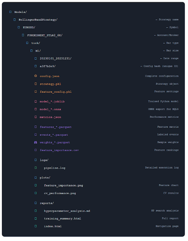
| ファイルの種類(色分けで区別) | 機能 |
|---|---|
| 設定ファイル | この実験を再現するために必要な設定をすべて記載します。設定ハッシュは一意性を保証します。 |
モデルファイル | 複数の形式で学習済みモデル:リサーチにはPython (joblib)、MQL5のデプロイにはONNXを使用。 |
データアーティファクト | 処理された特徴量、ラベル、および重み。再計算なしでモデル分析が可能になる。 |
レポートとログ | 包括的なドキュメント:実行ログ、パフォーマンスチャート、分析レポート。 |
この構成が提供するもの
- 簡単なナビゲーション:戦略、銘柄、日付範囲ごとに任意の実験を見つけられる
- 完全な再現性:設定ハッシュにより一意性とトレーサビリティが保証される
- 実験の比較:異なる設定を並べて比較できる
- 迅速な導入:MQL5 EAにドロップできるONNXファイル
- 完全な監査証跡:すべて自動的に文書化される
特定の条件に合致する学習済みモデルを見つけるには、以下のコードを使用できます。
from ..production.utils import ModelFileManager

file_manager = ModelFileManager()

base_dir = "Models"  # base_dir is path to where trained models are saved
search_criteria = {"bar_size": "M1", "bar_type": "time"}

file_manager.find_models(search_criteria, base_dir)
キャッシュの力
このシステムを高速にしている要因について説明します。この効率性の核心は、インテリジェントなキャッシュ無効化ロジックにあります。これは、変更が加えられた際に、パイプラインの必要なコンポーネントだけが再計算されることを保証します。機械学習のワークフローを依存関係グラフとして扱うことで、システムは、データシンボルの変更のような全ステージの完全な再計算を必要とする大きな変更と、モデルのハイパーパラメータ調整のような軽微な変更を区別できます。後者の場合、システムはバー、特徴量、ラベル、重みのキャッシュ済みデータを再利用し、最終的なモデル学習ステップのみを実行します。この粒度の高い制御により冗長な計算が防がれ、リサーチ者はデータセット全体を再処理することなく、特徴量エンジニアリングやラベリングなど特定部分に対して反復できるようになります。
より深く知りたい場合は、このシリーズの最後の記事を参照してください。
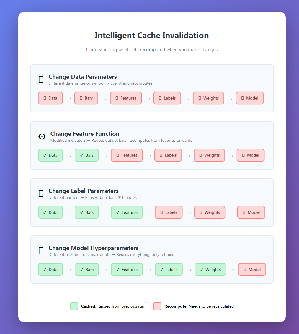
初回実行後、後続の実験は劇的に高速になります。
キャッシュの安全性とデータ汚染
最も重要な特徴は汚染防止です。すべてのデータアクセスがログに記録されます。
@cacheable(time_aware=True)
def load_and_prepare_training_data(...):
    # ... load data ...
    log_data_access(
            dataset_name=f"{symbol}_{bar_type}_{bar_size}".lower(),
            start_date=data.index[0],
            end_date=data.index[-1],
            purpose="train",
            data_shape=data.shape)

    return data
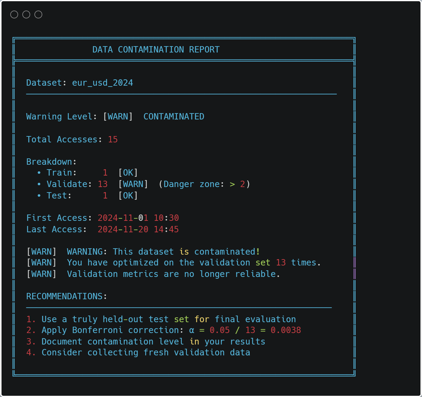
いつでも汚染の有無を確認できます。
from ..cache import print_contamination_report


print_contamination_report()
実践的な使用パターン
一般的なリサーチワークフローをいくつかご紹介しましょう。
1. 戦略の比較
strategies = [
        BollingerBandStrategy(window=20, num_std=2.0),
        BollingerBandStrategy(window=20, num_std=2.5),
        BollingerBandStrategy(window=30, num_std=2.0),
]
results = []

for strategy in strategies:
        pipeline = ModelDevelopmentPipeline(
                                symbol="EURUSD",
                                train_start="2023-01-01",
                                train_end="2023-12-31",
                                strategy=strategy,
                                # ... config ...
                )
        model, features, metrics, config = pipeline.run(verbose=False)
        results.append({
                        "strategy": strategy.get_strategy_name(),
                        "cv_score": metrics["cv_results"]["best_score"],
                        "features": len(features), "model": model
                })

comparison = pd.DataFrame(results).sort_values("cv_score", ascending=False)
print(comparison)
キャッシュのおかげで、戦略の比較は高速で、変更されるのはモデルの学習だけです。
2.特徴量エンジニアリング実験
feature_configs = [
        {"func": calculate_basic_features, "params": {}},
        {"func": calculate_advanced_features, "params": {"lookback": 20}},
        {"func": calculate_advanced_features, "params": {"lookback": 50}},
        ]

for i, feat_config in enumerate(feature_configs):
        pipeline = ModelDevelopmentPipeline(
			# ... same data config ... feature_config=feat_config,
			# ... rest of config ...
			)
        model, features, metrics, _ = pipeline.run()
	print(f"Feature set {i+1}: {metrics['cv_results']['best_score']:.4f}")
3. ウォークフォワード分析
train_periods = [
	("2022-01-01", "2022-12-31"),
	("2022-07-01", "2023-06-30"),
	("2023-01-01", "2023-12-31"),
	]
models = []

for train_start, train_end in train_periods:
        pipeline = ModelDevelopmentPipeline(
                                symbol="EURUSD",
                                train_start=train_start,
                                train_end=train_end,
                                # ... config ...
                                )
        model, _, metrics, _ = pipeline.run()
        models.append({
                        "period": f"{train_start} to {train_end}",
                        "score": metrics["cv_results"]["best_score"],
                        "model_path": pipeline.file_paths["model"]
                         })
整理されたディレクトリ構造により、異なる期間のモデルを容易に比較できます。
パフォーマンス監視
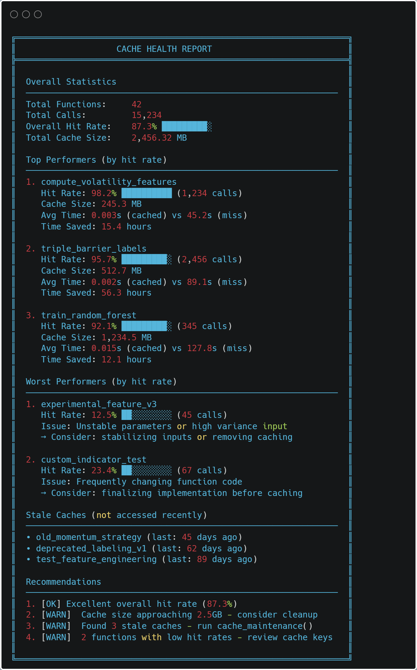
システムは自身のパフォーマンスを追跡します。
from ..cache import print_health_report

print_health_report()
MQL5との統合
ONNXエクスポート機能により、導入が容易になります。以下は、最小限のMQL5 EAの骨組みです。
//+------------------------------------------------------------------+
//|                                     BollingerBandStrategy_EA.mq5 |
//+------------------------------------------------------------------+

#property version   "1.00"
#property strict

//--- Include Resources
#include <Trade\Trade.mqh>

//--- Load the ONNX model from resources
#resource "\\Models\\BollingerBandStrategy\\EURUSD\\model.onnx" as uchar model_data[]

//--- Input Parameters
input double   InpLotSize      = 0.01;   // Trade Lot Size
input double   InpThresholdBuy = 0.55;   // Probability to Buy
input double   InpThresholdExit = 0.45;  // Probability to Exit/Sell

//--- Global Variables
long           model_handle    = INVALID_HANDLE;
CTrade         trade;

//+------------------------------------------------------------------+
//| Expert initialization function                                   |
//+------------------------------------------------------------------+
int OnInit()
{
    // Load ONNX model from the resource buffer
    model_handle = OnnxCreateFromBuffer(model_data, ONNX_DEFAULT);

    if(model_handle == INVALID_HANDLE)
    {
        Print("Error: Failed to load ONNX model. Code: ", GetLastError());
        return(INIT_FAILED);
    }

    // Set output shape if necessary (depends on your model export)
    // OnnxSetOutputShape(model_handle, 0, [1, 1]);

    Print("Model loaded successfully. Handle: ", model_handle);
    return(INIT_SUCCEEDED);
}

//+------------------------------------------------------------------+
//| Expert deinitialization function                                 |
//+------------------------------------------------------------------+
void OnDeinit(const int reason)
{
    if(model_handle != INVALID_HANDLE)
    {
        OnnxRelease(model_handle);
        model_handle = INVALID_HANDLE;
    }
}

//+------------------------------------------------------------------+
//| Expert tick function                                             |
//+------------------------------------------------------------------+
void OnTick()
{
    // 1. Prepare Features
    double features[47];
    if(!CalculateFeatures(features)) return;

    // 2. Prepare ONNX Vectors
    vector v_features;
    v_features.Assign(features);
    vector v_output;

    // 3. Run Inference
    if(!OnnxRun(model_handle, ONNX_NO_CONVERSION, v_features, v_output))
    {
        Print("Inference failed. Error: ", GetLastError());
        return;
    }

    // 4. Trade Logic
    double probability = v_output[0];
    CheckTradeLogic(probability);
}

//+------------------------------------------------------------------+
//| Logic for Entry and Exit                                         |
//+------------------------------------------------------------------+
void CheckTradeLogic(double prob)
{
    bool hasPosition = (PositionsTotal() > 0);

    // Buy Logic
    if(prob > InpThresholdBuy && !hasPosition)
    {
        trade.Buy(InpLotSize, _Symbol, SymbolInfoDouble(_Symbol, SYMBOL_ASK), 0, 0, "ONNX Signal");
    }
    // Exit Logic
    else if(prob < InpThresholdExit && hasPosition)
    {
        trade.PositionClose(_Symbol);
    }
}

//+------------------------------------------------------------------+
//| Feature Calculation - MUST MATCH PYTHON PRE-PROCESSING           |
//+------------------------------------------------------------------+
bool CalculateFeatures(double &features[])
{
    ArrayInitialize(features, 0.0);

    // Example: Getting Bollinger Bands data for the current bar
    double bb_upper = iBands(_Symbol, PERIOD_CURRENT, 20, 2.0, 0, PRICE_CLOSE, MODE_UPPER, 0);
    double bb_lower = iBands(_Symbol, PERIOD_CURRENT, 20, 2.0, 0, PRICE_CLOSE, MODE_LOWER, 0);
    double close    = iClose(_Symbol, PERIOD_CURRENT, 0);

    // Fill your 47 features here exactly as your model expects
    // features[0] = (close - bb_lower) / (bb_upper - bb_lower); // Normalized example
    // ...

    return true;
}
重要なのは、Pythonでの前処理と完全に一致する特徴量を確実に作ることです。学習のサマリーに含まれる特徴量リストが、その対応に役立ちます。
デバッグとトラブルシューティング
何らかの問題が発生した場合、システムは詳細な診断情報を提供します。
例:モデル性能の低下
# Get all experiments for a symbol
file_manager = ModelFileManager("Models")
models = file_manager.find_models({ "symbol": "EURUSD", "strategy": "BollingerBandStrategy" })

# Compare performance over time
for model_info in models:
        metrics = json.load(open(model_info["file_path"].replace(".joblib", "_metrics.json")))
        print(f"{model_info['date_range']}: {metrics['cv_results']['best_score']:.4f}")
パフォーマンスが変化した時期を素早く特定し、対応する設定を読み込むことで、何が変わったのかを確認できます。
例:キャッシュの問題
キャッシュの破損が疑われる場合:
from cache import clear_cache

# Clear specific function cache
clear_cache("load_and_prepare_training_data")

# Or clear everything
clear_cache()
システムは正確性を確保するために、ゼロから再構築されます。
ベストプラクティス
このシステムを数か月使用した後の私の感想は以下のとおりです。
1. 戦略名には必ず分かりやすい名前を使用する
# Good strategy name
BollingerBandStrategy(window=20, num_std=2.0)
strategy.get_strategy_name() # "BollingerBand_w20_std2.0"

# Better - includes your hypothesis strategy
BollingerBandStrategy(window=20, num_std=2.0, name="BB_MeanReversion_v1")
50件の実験を閲覧した時、未来のあなたはきっと感謝するでしょう。
2.小さなパラメータグリッドから始める
# First iteration - quick feedback
param_grid = {
	"n_estimators": [100, 200],
	"max_depth": [3, 5, 7]
	}

# After you understand the landscape
param_grid = {
	"n_estimators": [100, 200, 300, 500],
	"max_depth": [3, 5, 7, 10, 15],
	"min_samples_split": [2, 5, 10, 20]
	}
まずは迅速に反復作業をおこない、その後で洗練させていきます。
3. すべて保存する
ストレージは安価ですが、再現性はかけがえのないものです。
pipeline.run(
        generate_reports=True, # Always
        save=True, # Always
        export_onnx=True, # If deploying
        verbose=True # Until you're confident
        )
4. デプロイ前にレポートを確認する
CVスコアだけに基づいてデプロイしてはいけません。以下を確認します。
- フォールドの一貫性(ばらつきが大きいほど信頼性が低い)
- 特徴量の重要度(妥当な特徴量?)
- ラベルの分布(バランスが取れているか?)
- ONNX検証(合格?)
レポートを見れば簡単に確認できます。
5. 特徴量関数のバージョン管理
def calculate_features_v1(data, **params):
        """Initial feature set - baseline."""
        # ... features ...

def calculate_features_v2(data, **params):
        """Added momentum indicators."""
        # ... features ...

feature_config = { "func": calculate_features_v2, # Track version in function name
                   "params": {}
		}
特徴量を改善する際は、新しい関数を作成します。キャッシュはバージョン管理を自動的に処理します。
結論
本番運用レベルのリサーチシステムを構築するには初期投資が必要ですが、その効果は非常に大きいものです。
- スピード:同じ時間で10倍の実験が可能
- 信頼性:再現可能で信頼できる結果
- インサイト:自動分析により見落としがちなパターンを発見
- デプロイ:ワンボタンでMQL5へエクスポート
- 保守性:デバッグが容易で拡張も簡単
ここで紹介したコードは、金融機械学習リサーチ手法の中でも特に重要な要素を備えています。適切なクロスバリデーション、サンプル重み付け付け、特徴量分析(ただし非常に限定的)、検証といったベストプラクティスを強制的に適用し、「正しい方法を簡単に実行できる」ように設計されています。
最も重要なのは、取引戦略の改善という本質的な部分に集中できるようになることです。インフラ部分はすべて機能します。
次のステップ
このシステムを実装するためには以下の手順を推奨します。
- 小さく始める:単一の戦略と銘柄から開始
- キャッシュの検証:パイプラインを2回実行し、高速化を確認
- レポート確認:生成されたすべてのレポートをレビュー
- ONNX検証:予測が完全に一致することを確認
- 慎重にデプロイ:まずはペーパートレードで開始
- 反復改善:システムを使って体系的な実験を実施
完全なコードは付属ファイルに含まれています。まずはproductionフォルダ内の model_development.pyから始め、その後サンプルノートブックを確認してください。
忘れないでください。トレードはただでさえ難しいのですから、リサーチツールでさらに困難にするべきではありません。勝つためのシステムを構築しましょう。
ファイルリファレンスガイド
| ファイル | 主な目的 | 主要なクラス/関数 | 依存関係 | 用途 |
|---|---|---|---|---|
| __init__.py | モジュールのエクスポート | complete_export_workflow() export_model_to_onnx() extract_onnx_metadata() validate_onnx_predictions() | model_export.py | パッケージレベルでONNXエクスポート機能を公開 |
| dual_model_development.py | 買値/売値を考慮した、ロング/ショート別のモデル | BidAskLongShortPipeline train_bidask_longshort_models() | model_development.py、戦略クラス | 現実的な約定価格(ロングはask、ショートはbid)を用いて、買いポジションと売りポジションそれぞれに個別のモデルが必要な場合 |
| model_development.py | 中核パイプライン | ModelDevelopmentPipeline TickDataLoader load_and_prepare_training_data() generate_events_triple_barrier() train_model_with_cv() | feature_engine、sklearn、numba、キャッシュシステム | 完全な再現性を備えた、あらゆる単一モデルの学習と評価のための主要なパイプライン |
| model_export.py | ONNX変換と検証 | export_model_to_onnx() validate_onnx_predictions() complete_export_workflow() | skl2onnx、onnxruntime | MQL5デプロイ前の最終ステップ - 本番モデルがPythonと完全に一致することを確認 |
| utils.py | ファイル管理と整理 | ConfigPathGenerator ModelFileManager find_models() load_artifacts() | hashlib、json、pickle、pathlib | モデルディレクトリ構造の管理、成果物の保存/読み込み、過去の実験の検索 |
ファイル間の関係
- __init__.py → model_export.py(エクスポート関数を公開)
- dual_model_development.py → model_development.py(基本パイプラインを拡張)
- model_development.py → utils.py(ファイル管理を使用)
- model_export.py → スタンドアロン(単独で動作可能)
- すべてのファイル → キャッシュシステム(パフォーマンス向上のため)
主な統合ポイント
- dual_model_development.pyは、2 つの ModelDevelopmentPipelineインスタンス(ロング/ショート)を作成
- utils.pyのModelFileManagerは、ModelDevelopmentPipelineによって整理されたストレージとして使用
- export_model_to_onnx()は、export_onnx=True の場合にModelDevelopmentPipelineから呼び出される
MetaQuotes Ltdにより英語から翻訳されました。
元の記事: https://www.mql5.com/en/articles/20451
警告: これらの資料についてのすべての権利はMetaQuotes Ltd.が保有しています。これらの資料の全部または一部の複製や再プリントは禁じられています。
この記事はサイトのユーザーによって執筆されたものであり、著者の個人的な見解を反映しています。MetaQuotes Ltdは、提示された情報の正確性や、記載されているソリューション、戦略、または推奨事項の使用によって生じたいかなる結果についても責任を負いません。

 ラリー・ウィリアムズの『市場の秘密』(第10回):スマッシュデー反転パターンの自動化
 バックトラッキング探索アルゴリズム(BSA)
 カスタムインジケータワークショップ(第2回):MQL5で実用的なSupertrend EAを構築する
 プライスアクション分析ツールキットの開発(第29回):Boom and Crash Interceptor EA

- 無料取引アプリ
- 8千を超えるシグナルをコピー
- 金融ニュースで金融マーケットを探索