How to Train an MLP Using Markov Chain Features in MQL5

Introduction

In this article, we will systematically construct a regime-dependent market model based on a Markov chain and a multilayer perceptron (MLP). Instead of feeding a price series directly into a neural network, we will first give market behavior a mathematical structure: the market will be represented as a Markov chain with three states describing different market phases. We will examine why a three-state model was chosen, how a vector of 15 probabilistic features is formed from the chain’s transitions, and how these features are used to train an MLP, followed by validation on a holdout set.

Next, we will examine the model's results, compare it with baseline approaches, and discuss its practical implementation in the form of the Markov_MLP_Oscillator.mq5 indicator. At the end of this article, we will provide recommendations on how to configure the parameters and use the model in real trading conditions.

Problem Statement

Most machine learning indicators for trading feed raw data — such as prices, volumes, and RSI and MACD values — into a neural network. The model does not receive an explicit description of the market phase — it attempts to reconstruct it from a stream of numbers. As a result, it is more difficult for a neural network to extract context directly from a price series, and the quality of the signals may be inconsistent.

The problem runs deeper than it seems. If the closing prices of EURUSD for the last 100 bars are fed into the neural network, the model is expected to reconstruct the context on its own: to distinguish a sideways market from an impulsive move and recognize trend continuation after consolidation. The network finds it difficult to do this from closing prices alone: the same values have different meanings in a trending market and a sideways market. It is like asking someone to predict the weather by showing them only thermometer readings — without air pressure, humidity, or wind direction.

In this article, the approach changes. First, the market is described mathematically — using a Markov chain with three states. The MLP then predicts price direction based solely on the probabilistic features generated by the chain. The network does not receive the original price series as input, but rather a structured probabilistic description of the market.

Readers will get:

• the ready-to-use Markov_MLP_Oscillator.mq5 indicator, featuring an oscillator, a color histogram, and a smoothed signal;
• the CMarkovChain class — an independent, reusable module;
• the CMLP class — a minimalist perceptron with backpropagation, written entirely in MQL5;
• a validation scheme using a held-out sample, with accuracy reporting;
• an architecture that uses a chain as a preprocessor and can be applied to any set of Markov states.

Markov Chain

A Markov chain is a mathematical model proposed by A.A. Markov in 1906. At any given moment, the system is in one of the states of a finite set. Key property: the probability of transitioning to the next state depends only on the current state, not on the entire history leading up to it. This property is called memorylessness.

Formally, if we denote the state of the system at time t as Sₜ:

P(Sₜ₊₁ = j | Sₜ = i, Sₜ₋₁, ..., S₀) = P(Sₜ₊₁ = j | Sₜ = i) = pᵢⱼ

All transition probabilities pᵢⱼ form the transition matrix P. Each row of the matrix sums to 1. This matrix serves as the chain's memory of the behavior of the process under study.

Three Market States

Why not two?

Using only two states (up/down) fails to capture the neutral zone: a flat market, consolidation, or low-volatility sideways trading. This is the area that provides the most useful information for filtering signals — it is best to refrain from trading here. With two possible states, the model is forced to take a position in every case, which leads to an excessive number of trades.

Why not five or more?

As the number of states increases, so do the dimensions of the transition matrix and the number of parameters. With a limited history (1,000–2,000 bars), each row of the matrix is updated infrequently, and the probabilities become less stable. Three states provide an optimal balance between informativeness and the statistical reliability of the estimates.

Limitations of the three-state model

• Using three states is a simplification. The model does not distinguish between strong and weak trends.
• Volatility is not taken into account.
• The model is a decision-making tool, not an exact description of the market.

Three states are used to describe the market:

• State 0 — downtrend: the price has fallen by more than a specified threshold in points over the last N bars.
• State 1 — flat: the price has changed only slightly over the last N bars.
• State 2 — uptrend: the price has risen by more than a specified threshold over the last N bars.

The transition matrix is a 3×3 matrix:

From \ To	Down (0)	Flat (1)	Up (2)
Down (0)	p₀₀	p₀₁	p₀₂
Flat (1)	p₁₀	p₁₁	p₁₂
Up (2)	p₂₀	p₂₁	p₂₂

Each element pᵢⱼ indicates the probability that the market will transition from phase i to phase j in the next step.

N-step forecast

A Markov chain allows us to make predictions not only one step ahead, but also N steps ahead. The initial probability vector is multiplied by the transition matrix N times:

v(t+N) = v(t) × Pᴺ

If the current state is known exactly (for example, "Up"), the initial vector is v = [0, 0, 1]. Multiplying the initial vector by matrix P N times yields the probability distribution across all three states after N steps. This distribution becomes part of the feature vector for the MLP.

As N increases, the probabilities smooth out and tend toward the stationary distribution of the chain. Practical range for trading: N from 2 to 5.

Entropy as a measure of uncertainty

One of the features is normalized Shannon entropy:

H = -∑ pᵢ · log(pᵢ) / log(N_states)

• H ≈ 0: The probabilities are concentrated in a single state — the market regime is well defined.
• H ≈ 1: All three states are approximately equally likely — the market is in a transitional state.

This feature indicates to the MLP how confident the chain itself is in its current forecast.

Indicator Architecture

The system operates in two stages.

• Stage 1 — Markov chain. It accumulates transition statistics from historical data, constructs the matrix P, and generates a feature vector for each bar.
• Stage 2 — MLP classifier. It is trained to predict the label (whether the price will be higher or lower HORIZON bars ahead) based solely on Markov features.

It is crucial to note that the MLP does not receive the original price series as input, but rather a probabilistic description of market states. Price is used solely for two auxiliary purposes: constructing the transition matrix and generating training labels.

Architecture Diagram

Price history
    │
    ▼
GetPhase(): discretization to {0, 1, 2} states
    │
    ▼
Build(): P transition matrix (3×3, Laplace smoothing)
    │
    ├──► Probs1Step()  → P(Down), P(Flat), P(Up) | 1 step
    ├──► ProbsNStep()  → P(Down), P(Flat), P(Up) | N steps
    ├──► LaggedStates() → states t-1, t-2, ..., t-L
    └──► ShannonEntropy() → H₁, Hₙ
                │
                ▼
        Feature vector (15 values)
                │
                ▼
          MLP (15 → 24 → 2)
                │
                ▼
        P(Bull), P(Bear)
                │
                ▼
  Oscillator = P(Bull) − P(Bear)

Feature vector

With the default settings (MC_LAG_COUNT = 4), each bar is described by 15 features:

Index	Feature	Meaning
[0]	P(Down | cur)	Probability of transitioning to the down state in one step
[1]	P(Flat | cur)	One-step probability of transitioning to the flat state
[2]	P(Up | cur)	One-step probability of transitioning to the up state
[3]	P(Up) − P(Down)	One-step directional signal
[4]	State / 2	Normalized state: 0.0 / 0.5 / 1.0
[5]	P(Down, N steps)	Probability of being in the Down state after N steps
[6]	P(Flat, N steps)	Probability of being in the Flat state after N steps
[7]	P(Up, N steps)	Probability of being in the Up state after N steps
[8]	P(Up) − P(Down), N steps	Directional signal after N steps
[9–12]	State lags	4 previous market states (normalized)
[13]	Entropy H₁	Uncertainty in the 1-step distribution
[14]	Entropy Hₙ	Uncertainty in the N-step distribution

MLP Architecture:

Input layer (15 neurons)
    → Hidden layer (24 neurons, ReLU)
    → Output layer (2 neurons, Softmax)

Training uses stochastic gradient descent, with the training data shuffled at each epoch. Weights are initialized using He initialization, with a standard deviation of √(2/n_in).

Generating training labels

For each bar t, a binary label is generated based on the price movement HORIZON bars ahead. To filter out noisy examples with negligible price movement, a threshold δ is applied:

y(t) = 1 (Bull),  if Close[t + HORIZON] − Close[t] >  δ
y(t) = 0 (Bear),  if Close[t + HORIZON] − Close[t] < −δ
y(t) = skip if |Close[t + HORIZON] − Close[t]| ≤ δ

By default, δ = 0 (all bars are included in training). For stricter labeling, δ should be set to 5–15 points for EURUSD H1. This reduces the number of training examples, but also reduces the noise in the labels.

Implementation in MQL5

Determining the Market State

The GetPhase method determines the current market state based on price movement over the number of bars specified by the period parameter:

//+------------------------------------------------------------------+
//| Determine the market phase at bar shift                          |
//| Returns: 0=DownTrend, 1=Flat, 2=UpTrend                          |
//+------------------------------------------------------------------+
int GetPhase(int shift, int period, double threshold)
  {
   double cn[], cp[];
   //--- Load the closing prices of the current bar and the bar period bars ago
   if(CopyClose(_Symbol, _Period, shift,        1, cn) <= 0) return(1);
   if(CopyClose(_Symbol, _Period, shift + period, 1, cp) <= 0) return(1);
   //--- price movement in points: positive = rise, negative = fall
   double move = (cn[0] - cp[0]) / _Point;
   if(move >  threshold) return(2);  // upward trend
   if(move < -threshold) return(0);  // downward trend
   return(1);                        // flat
  }

Building a Transition Matrix

The Build method iterates through the history, counts the observed transitions, and normalizes the rows. Laplace smoothing (initial count = 1) ensures that no probability is zero:

//+------------------------------------------------------------------+
//| Build transition matrix from history [fromShift..toShift]        |
//| Laplace smoothing (initial count=1) prevents zero probabilities  |
//+------------------------------------------------------------------+
void Build(int fromShift, int toShift, int period, double threshold)
  {
   //--- Initialize counters with Laplace smoothing
   for(int i = 0; i < MC_STATES; i++)
      for(int j = 0; j < MC_STATES; j++)
         m_counts[i][j] = 1.0;

   //--- Count transitions: from older bars to newer bars
   for(int shift = toShift; shift > fromShift; shift--)
     {
      int from = GetPhase(shift,     period, threshold);  // state at step t
      int to   = GetPhase(shift - 1, period, threshold);  // state at step t+1
      m_counts[from][to] += 1.0;
     }

   //--- Normalize the rows: the sum of each row equals 1.0
   for(int i = 0; i < MC_STATES; i++)
     {
      double rowSum = 0.0;
      for(int j = 0; j < MC_STATES; j++) rowSum += m_counts[i][j];
      for(int j = 0; j < MC_STATES; j++)
         m_probs[i][j] = m_counts[i][j] / rowSum;
     }
  }

N-step forecast

The ProbsNStep method implements the iterative multiplication of a probability vector by a transition matrix. The initial vector is a one-hot vector representing the current state; after N iterations, out[] contains the probability distribution after N steps:

//+------------------------------------------------------------------+
//| Forecast probability distribution after N steps                  |
//| Input:  state — current market state (0/1/2)                     |
//| Output: out[] — probability distribution over 3 states           |
//+------------------------------------------------------------------+
void ProbsNStep(int state, int steps, double &out[])
  {
   //--- Initialization: probability 1.0 in the current state, 0.0 in all other states
   double vec[MC_STATES];
   for(int j = 0; j < MC_STATES; j++)
      vec[j] = (j == state) ? 1.0 : 0.0;

   //--- Multiply a vector by a matrix N times: vec = vec × P
   for(int s = 0; s < steps; s++)
     {
      double nv[MC_STATES];
      ArrayInitialize(nv, 0.0);
      for(int j = 0; j < MC_STATES; j++)
         for(int i = 0; i < MC_STATES; i++)
            nv[j] += vec[i] * m_probs[i][j];
      for(int j = 0; j < MC_STATES; j++) vec[j] = nv[j];
     }

   ArrayResize(out, MC_STATES);
   for(int j = 0; j < MC_STATES; j++) out[j] = vec[j];
  }

Forming a feature vector

The GetFeatures function assembles the complete feature vector for a single bar. Four groups of features (A–D) cover the current state, short-term and multi-step forecasts, the historical sequence of states, and a measure of uncertainty:

//+-------------------------------------------------------------------------------------+
//| Build a Markov feature vector for one bar                                           |
//| Groups A–D: 1-step probabilities, N-step probabilities, lagged states, entropies    |
//| Return 'false' if there is not enough history for all lag lookbacks                 |
//+-------------------------------------------------------------------------------------+
bool GetFeatures(int bar_idx, RawFeatures &feat, CMarkovChain &mc, int nRaw)
  {
   int total = Bars(_Symbol, _Period);
   //--- Check that bars are available for all lagged states
   if(bar_idx + MC_TREND_PERIOD * (MC_LAG_COUNT + 2) + 5 >= total) return(false);

   int curState = mc.GetPhase(bar_idx, MC_TREND_PERIOD, MC_TREND_PIPS);

   //--- Group A: 1-step transition probabilities + directional signal + state
   double p1[];
   mc.Probs1Step(curState, p1);
   feat.v[0] = p1[0];          // P(Down | cur)
   feat.v[1] = p1[1];          // P(Flat | cur)
   feat.v[2] = p1[2];          // P(Up | cur)
   feat.v[3] = p1[2] - p1[0];  // directional signal: bullish pressure minus bearish pressure
   feat.v[4] = curState * 0.5; // 0.0=Down, 0.5=Flat, 1.0=Up

   //--- Group B: N-step probabilities + directional signal
   double pN[];
   mc.ProbsNStep(curState, MC_STEPS, pN);
   feat.v[5] = pN[0];          // P(Down after N steps)
   feat.v[6] = pN[1];          // P(Flat after N steps)
   feat.v[7] = pN[2];          // P(Up after N steps)
   feat.v[8] = pN[2] - pN[0];  // directional signal after N steps

   //--- Group C: lagged states (compensate for Markovian memorylessness)
   for(int lag = 1; lag <= MC_LAG_COUNT; lag++)
     {
      int lagShift = bar_idx + lag * MC_TREND_PERIOD;
      int lagState = mc.GetPhase(lagShift, MC_TREND_PERIOD, MC_TREND_PIPS);
      feat.v[8 + lag] = lagState * 0.5;  // normalized past state
     }

   //--- Group D: Shannon entropy—a measure of forecast uncertainty
   int eIdx = 9 + MC_LAG_COUNT;
   feat.v[eIdx]     = ShannonEntropy(p1, MC_STATES); // uncertainty of the 1-step forecast
   feat.v[eIdx + 1] = ShannonEntropy(pN, MC_STATES); // uncertainty of the N-step forecast

   return(true);
  }

Training and Validation Procedure

The data is divided by time: the older bars constitute the training set, and the newer ones constitute the validation set. This simulates real trading: the model is trained on past data and evaluated on later data that is already available historically.

//+-----------------------------------------------------------------------+
//| Split data: 80% oldest = training, 20% newest = validation            |
//| Time-correct split: train on past data, validate on more recent data  |
//+-----------------------------------------------------------------------+
int trainN = (int)MathFloor(cnt * 0.80);
if(trainN < 80) trainN = cnt;
int valN = cnt - trainN;

//--- Step 1: Train the model on the trainN oldest samples
//--- Step 2: Evaluate on the valN newest samples → g_validationAccuracy
//--- Step 3: The final model is trained on all cnt samples

After evaluation, the final model is trained on all cnt samples — this provides the most up-to-date picture of the current market state.

Is an MLP needed on top of a Markov chain?

Before adding a neural network, it is a good idea to make sure that it actually improves the results compared to simpler approaches.

The directional signal of the chain itself — P(Up) − P(Down) — is already a fully functional oscillator without any training. The MLP adds a nonlinear combination of 15 features, including entropy, lagged states, and N-step forecasts. This potentially allows us to identify patterns that a simple difference signal does not capture.

Indicative results (EURUSD H1, 2023–2024)

The table below illustrates the approximate level of accuracy using EURUSD H1 as an example. The specific values depend on the time period, chain parameters, and the forecast horizon.

Model	EURUSD H1	GBPUSD H1	XAUUSD M15
MLP trained on raw closing prices	~51%	~51%	~50%
MLP trained on RSI/MACD	~53%	~52%	~51%
Markov chain only (P(Up) − P(Down))	~54%	~53%	~52%
Markov Chain → MLP	~57%	~55%	~53%

If, for a specific instrument and timeframe, Markov Chain → MLP is no more accurate than a simple Markov signal, you should review the chain’s parameters (MC_TREND_PERIOD, MC_TREND_PIPS) or the forecast horizon.

Note. A 57% accuracy rate is no guarantee of profit: it merely indicates that the model detects patterns in the data. Actual trading performance depends on commissions, slippage, and risk management.

Indicator Parameters

Parameter	Default	Description
HORIZON	24	Forecast horizon: the number of bars after which the label is determined
LOOKBACK	2000	Historical lookback for training (bars)
RETRAIN_EVERY	24	Retraining every N new bars
MLP_HIDDEN	24	Number of neurons in the hidden layer
MLP_LR	0.0001	Learning rate
MLP_EPOCHS	400	Number of training epochs for an MLP
SIGNAL_THRESH	0.25	Confidence threshold for histogram coloring
CLOSED_BAR_ONLY	true	Calculation on closed bars only
SMOOTH_PERIOD	5	Output signal smoothing period
MC_TREND_PERIOD	10	Number of bars over which price movement is measured to determine the state
MC_TREND_PIPS	20	Price movement threshold in points for determining the trend
MC_STEPS	3	Horizon of an N-step chain forecast
MC_LAG_COUNT	4	Number of lagged states used as features

Configuration Recommendations

The MC_TREND_PERIOD and MC_TREND_PIPS parameters determine the chain's sensitivity to market movements. For EURUSD on the H1 timeframe, use 10 bars and 20 points. For D1, the threshold should be increased to 100–150 points; otherwise, every daily bar will be identified as a trend, and the transition matrix will lose its informational value.

The MC_LAG_COUNT parameter introduces memory of past states, partially compensating for the Markov property of memorylessness. Values of 3–6 offer a good balance between information content and the risk of overfitting.

HORIZON is selected based on the typical duration of a market move. To capture intraday price movements lasting 4–6 hours on the H1 timeframe, it makes sense to set HORIZON = 4–6.

The Risk of Overfitting

When MLP_EPOCHS = 400 and the historical data is limited (1,000–2,000 bars), there is a risk of the model being overfitted to a specific segment of the data. Signs of overfitting:

• The accuracy on the training set is significantly higher than on the validation set;
• Signals fluctuate erratically when there is a slight change in MC_TREND_PIPS or HORIZON;
• An overfitted model stops working when the market regime changes.

To reduce the risk, it is recommended to decrease MLP_EPOCHS to 150–250 or increase LOOKBACK.

Using the Signal in Trading

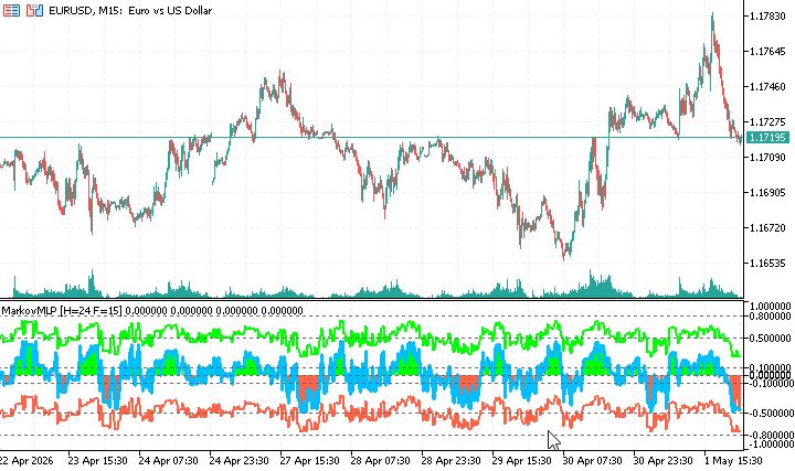
The output signal is the difference P(Bull) − P(Bear), normalized to the range [−1, +1]:

• Green histogram (Osc > SIGNAL_THRESH): The MLP is fairly confident in the bullish scenario.
• Red histogram (Osc < −SIGNAL_THRESH): The MLP is fairly confident in the bearish scenario.
• Gray histogram: uncertainty; it is best to refrain from making a trade.

The blue Smooth Signal line is a smoothed version of the oscillator. When it crosses the zero line from below while the histogram is green, it provides additional confirmation of the bullish signal.

Diagnostic information in Comment

The following information is displayed in real time in the upper-left corner of the chart:

• current market state: DOWN TREND / FLAT / UP TREND;
• the probabilities of a 1-step transition and an N-step forecast;
• a 3×3 transition matrix;
• the classifier's accuracy on the validation set;
• the date of the last retraining.

Comparison of Approaches

Approach	MLP Input Data	Interpretability	Potential Noise Robustness
Raw OHLCV	Direct Price/Volume Inputs	Low	Low
Technical Indicators	RSI, MACD, MA, etc.	Medium	Medium
Naive Bayes → MLP	Bayesian Probabilities	Medium	Medium
Markov Chain → MLP	Phase Transition Probabilities	High	Potentially high

The main advantage of the Markovian approach is the interpretability of the features. A trader can view the Comment output to see the current market state, the probability of continuation, the entropy level, and the system's confidence level. This is fundamentally different from the "black box" of conventional deep learning.

Limitations

The transition matrix is built from historical data. If the market regime changes abruptly, the matrix will reflect the past. The RETRAIN_EVERY parameter helps, but it does not completely resolve this issue.

A validation accuracy of over 55–60% is a good sign. About 50% means that the system is not detecting patterns on this instrument or timeframe with the current settings. In this case, you should change MC_TREND_PERIOD, MC_TREND_PIPS, or HORIZON.

Conclusion

This article examines a two-level architecture for a trading indicator: the Markov chain is used not as a standalone forecasting tool, but as a generator of structured probabilistic features for a neural network.

Key principle: The quality of the features is more important than the complexity of the model. An MLP with a single hidden layer (24 neurons), trained on 15 Markov features, is sometimes more effective than a deep network trained on raw prices because it receives a meaningful description of market states. This is a principle that applies far beyond the scope of this article.

Another important point is interpretability. Unlike most ML indicators, the system shows at any given moment why it generated a particular signal: the current market state, transition probabilities, the 3×3 matrix, and the entropy of the distribution.

We recommend starting testing on EURUSD H1 with the default parameters, checking the validation accuracy in the Comment output, and then adjusting MC_TREND_PERIOD, MC_TREND_PIPS, and MC_LAG_COUNT to suit your instrument. If the accuracy during validation is close to 50%, this is a sign that the selected chain parameters do not capture the structure of this particular market on this timeframe. Change the thresholds, period, and horizon — and watch how the transition matrix changes in Comment.

Future areas of development: increasing the number of states in the chain (5–7 instead of 3), adaptively updating the transition matrix in a sliding window, combining multiple chains with different periods into a single feature vector, and using hidden Markov models (HMMs) instead of a standard chain.