

Neural Networks in Trading: Bidirectional Adaptive Temporal Correlation (Conclusion)
 119
 6

Introduction
The market has its own unique dynamics, and every movement is a burst of events — an instantaneous imprint of a shift in supply and demand. And the deeper we delved into the concept of event representations, the clearer it became that the BAT architecture seemed to have been designed specifically for this type of data. Its roots lie in the world of event-based vision, but its underlying logic is surprisingly well suited to the market. There are no frames here. There are only asynchronous streams — irregular, unpredictable, and infinitely varied. These streams must not merely be captured, but understood, structured, and turned into guides for decision-making.
We began by trying to identify the same structure in market movements that the authors of BAT find in the data stream from event cameras. And the voxel-grid concept they use aligns surprisingly well with our approach to handling financial data. In the original work, disorganized event noise is transformed into a dense, neatly organized cube of data. In it, time and space are woven into a single matrix. The same thing happens here, too. Ticks, volume spikes, and order book responses — we organize them into small temporal layers, transforming a chaotic stream into a structured grid that allows the model to operate on a solid foundation.
As a next step, BAT offers a multiscale view of movement. The market operates on several levels at once: in tiny price movements, in broad trend fluctuations, and in transitions between phases of volatility. And, like a seasoned analyst, the BAT architecture broadens its perspective by examining data from multiple angles simultaneously. It is delicate work. Small impulses often serve as the catalysts for large movements, while large shifts can mask microsegments of activity. Breaking the data down into multiple scales allows the framework to capture these transitions and form a more comprehensive view of the market.
However, the true power of BAT becomes apparent when the model begins to correlate events over time. The authors suggest using bidirectional temporal correlation — a concept very familiar to anyone who has ever tried to get a feel for the market in real time. To understand the current momentum, it is not enough to look only ahead. We need to see how the past connects with the future. Which structures remain stable, and which ones break down? BAT constructs a correlation tensor — a dense space that shows how well different time segments align with one another. The result is something like a map of market forces, where general trends, confirmations, divergences, and local distortions are evident.
But movement is never uniform. The pace of the market fluctuates — from a calm, slow flow to bursts of activity where milliseconds determine the outcome of a trade. It is precisely for these regimes that BAT uses adaptive temporal sampling, which can automatically adjust the analysis step size to match the nature of the current movement. When the market picks up speed, the model compresses time so as not to miss important transitions. Conversely, when the market quiets down, the model widens the time window, smoothing out the noise. As a result, the data stream is analyzed as if the system truly senses the market's rhythm, adapting to every new surge or lull.
Next, spatially adaptive aggregation comes into play. This is a form of feature cleaning and organization, where attention is focused not on all the data at once, but on those parts that actually drive the movement. BAT filters out outliers, discards inconsistent signals, and combines consistent elements into a single, stable representation of the dynamics. What we perceive in the market as a clear price bias or a strengthening trend materializes here as a Motion-Feature — a dense structure that reflects the true direction of movement.
Finally, the architecture uses iterative refinement to improve the motion estimate step by step. Just like an artist who first sketches the outline, then renders the form, light, and shadow. Each iteration makes the movement smoother, more precise, and more consistent, until the result is a reliable, fully developed solution. For the market, this means one thing: the model is able to view price movement as a structured process in which every impulse has its place and significance.
It is precisely this kind of architecture — sequential, multi-layered, and attentive to detail — that formed the basis of our own solution using MQL5 tools. We create events, form temporal layers, establish correlations, adjust the time step, and organize dynamics into coherent structures. This is not simply a matter of transferring an idea from one field to another, but rather an organic adaptation of a technology that was originally developed in the world of asynchronous data. The market is also an event camera — only it measures liquidity rather than light. And BAT turned out to be a surprisingly accurate tool that allows us to look deeper. See not just the price, but its movement, context, and structure.
The author's visualization of the BAT framework is shown below.


Top-level Object
In our previous work, we have already presented our own approach to implementing the key elements of the BAT framework and examined, one by one, the logic behind event-based data preparation, multiscale encoding, temporal correlation, and dynamic modeling. Each component was a separate step, like a single stroke in a larger picture. Now is the time to bring the entire system together into a single, integrated whole that can function as a cohesive mechanism. That is precisely why our implementation includes a top-level object designed to integrate data preparation, feature engineering, contextual modeling, and the final aggregation of dynamics into a single architectural framework.
The CNeuronBAT class, built as an extension of the event-based convolutional block, serves as this integration point. This is not just a control wrapper, but a fully-fledged framework in which all previous ideas find their place. It combines the stages of preparing the voxel representation, encoding market events, establishing temporal relationships, and subsequently reconstructing movement, forming a data processing flow from the first tick to the final impulse.
class CNeuronBAT :  public CNeuronSpikeConvBlock
  {
protected:
   CLayer                              cPrepare;
   CLayer                              cEncoder;
   CLayer                              cContext;
   CNeuronBaseOCL                      cConcatenated;
   CNeuronSpikeConvGRU2D               cGRU;
   CNeuronTransposeRCDOCL              cTranspose;
   //---
   virtual bool      feedForward(CNeuronBaseOCL *NeuronOCL) override;
   virtual bool      updateInputWeights(CNeuronBaseOCL *NeuronOCL) override;
   virtual bool      calcInputGradients(CNeuronBaseOCL *NeuronOCL) override;

public:
                     CNeuronBAT(void) {};
                    ~CNeuronBAT(void) {};
   //---
   virtual bool      Init(uint numOutputs, uint myIndex, COpenCLMy *open_cl,
                          uint dimension, uint embed_size,
                          uint stack_size, uint variables,
                          ENUM_OPTIMIZATION optimization_type, uint batch);
   //---
   virtual int       Type(void)   override const   {  return defNeuronBAT;   }
   //--- methods for working with files
   virtual bool      Save(int const file_handle) override;
   virtual bool      Load(int const file_handle) override;
   //---
   virtual bool      WeightsUpdate(CNeuronBaseOCL *source, float tau) override;
   //---
   virtual void      SetOpenCL(COpenCLMy *obj) override;
   virtual void      TrainMode(bool flag) override;
   virtual bool      Clear(void) override;
   virtual CBufferFloat   *getWeights(void) override;
  };
The main functional units are concentrated within this object. The cPrepare data preparation module is responsible for the initial structuring of events — a sort of market camera obscura that transforms raw ticks into a neatly layered event volume. Next comes cEncoder, which generates a multiscale representation that allows the model to see what lies between volatility transitions and local bursts of activity. Working in conjunction with it is cContext, which is responsible for constructing bidirectional temporal correlations and forming a contextual space in which the model identifies stable relationships between signals.
The cConcatenated node plays a special role, combining data from different processing levels; the entire data stream then flows into cGRU — a two-dimensional event-based GRU block that serves as the heart of dynamic modeling. It is precisely here that the smoothing, refinement, and accumulation of the temporal structure — which is so essential for identifying the true direction of market movement — take place.
As we moved on to assembling a fully functional BAT module, it became clear that all our previous work had merely been preparation for creating a unified mechanism in which each element occupies its own strictly designated place. At the same time, the entire structure works like clockwork. In financial markets, where even the slightest delay or distortion in signal processing can prove costly, such architectural coherence is not merely a nice-to-have but a necessity. Therefore, in our top-level BAT object, we carefully assemble the entire technology stack, integrating individual components into a cohesive neural network section designed to analyze temporal dependencies, contextual relationships, and nonlinear market structures.
bool CNeuronBAT::Init(uint numOutputs, uint myIndex, COpenCLMy *open_cl,
                      uint dimension, uint embed_size,
                      uint stack_size, uint variables,
                      ENUM_OPTIMIZATION optimization_type, uint batch)
  {
   if(!CNeuronSpikeConvBlock::Init(numOutputs, myIndex, open_cl, dimension, dimension,
                                   dimension, stack_size * variables, 1, optimization_type, batch))
      return false;
First, the base SpikeConvBlock is initialized — a sort of foundation through which all subsequent computations pass. It specifies the dimensions and optimization methods and ensures strict adherence to the computational topology. Only after the model's basic geometry has been securely established does the formation of the inner layers begin.
The data preparation module serves as the starting point for processing the quotes being analyzed. It includes normalization, through which the data passes in the same way that a traditional trader runs a stream of market values through checks, filters, and additional calculations before making a decision.
   int index = 0;
   CNeuronBatchNormOCL*                norm = NULL;
   CNeuronCreateFlow*                  stack = NULL;
   CNeuronSpikeConvBlock*              conv = NULL;
   CNeuronMultiWindowsConvWPadOCL*     mwconv = NULL;
   CNeuronMSRes*                       resblock = NULL;
   CNeuronBiDirectCorrelation*         correlation = NULL;
   CNeuronSATMA*                       satma = NULL;
//---
   cPrepare.Clear();
   cPrepare.SetOpenCL(OpenCL);
   norm = new CNeuronBatchNormOCL();
   if(!norm ||
      !norm.Init(0, index, OpenCL, dimension * variables, iBatch, optimization) ||
      !cPrepare.Add(norm))
     {
      DeleteObj(norm)
      return false;
     }
But the main action takes place a little further on. We create the CreateFlow component — a mechanism that converts discrete market sequences into a stream of spikes. This is not merely a formal format conversion, but a shift to an event-based representation of the data. Here, even the slightest price change becomes a brief electrical click. This representation makes the model more sensitive to market microstates and allows it to capture even the slightest fluctuations more accurately — fluctuations that often determine the outcome of a short-term trade.
   index++;
   stack = new CNeuronCreateFlow();
   if(!stack ||
      !stack.Init(0, index, OpenCL, stack_size, dimension, embed_size,
                                   variables, optimization, iBatch) ||
      !cPrepare.Add(stack))
     {
      DeleteObj(stack)
      return false;
     }
To prevent this spike stream from breaking down into isolated events, we build a stack of historical data that serves as the voxel tensor proposed by the framework's authors. In this structure, each time step becomes a layer, and each unitary sequence becomes a separate face. The result is a compact yet surprisingly informative representation of the market context that helps the network perceive the spatial structure of market states. In it, local spikes and global trends coexist side by side.
The system then proceeds step by step to build the Encoder and Context branches — two parallel branches that will later merge and complement each other, forming a comprehensive understanding of what is happening in the market. Both branches are initialized with a set of windows of different sizes: the base embed size and three, five, and seven times that size. This approach is a classic technique of multiscale convolution, which allows the model to consider both local fluctuations and broader market wave structures simultaneously. In trading, this is comparable to analyzing minute, hourly, and daily charts simultaneously: each provides its own insights, and only the overall picture reveals the market’s full intent.
   cEncoder.Clear();
   cContext.Clear();
   cEncoder.SetOpenCL(OpenCL);
   cContext.SetOpenCL(OpenCL);
//---
   uint windows[] = {embed_size, 3 * embed_size, 5 * embed_size, 7 * embed_size};
   mwconv = new CNeuronMultiWindowsConvWPadOCL();
   index++;
   if(!mwconv ||
      !mwconv.Init(0, index, OpenCL, windows, embed_size, embed_size, stack_size,
                                              variables, optimization, iBatch) ||
      !cEncoder.Add(mwconv))
     {
      DeleteObj(mwconv)
      return false;
     }
   mwconv.SetActivationFunction(None);
   mwconv = new CNeuronMultiWindowsConvWPadOCL();
   index++;
   if(!mwconv ||
      !mwconv.Init(0, index, OpenCL, windows, embed_size, embed_size, stack_size,
                                              variables, optimization, iBatch) ||
      !cContext.Add(mwconv))
     {
      DeleteObj(mwconv)
      return false;
     }
   mwconv.SetActivationFunction(None);
After initial processing, the branches gradually taper. To achieve this, cascades of MS-Res blocks and SpikeConv modules are created to reduce the number of windows. This is not merely a technical detail, but a well-thought-out, step-by-step compression process, similar to how an analyst gradually forms a consolidated view by filtering out noise and focusing on structural changes in price.
   uint mult = windows.Size();
   while(mult > 1)
     {
      index++;
      resblock = new CNeuronMSRes();
      if(!resblock ||
         !resblock.Init(0, index, OpenCL, mult * stack_size, embed_size, variables,
                                                           optimization, iBatch) ||
         !cEncoder.Add(resblock))
        {
         DeleteObj(resblock)
         return false;
        }
      index++;
      resblock = new CNeuronMSRes();
      if(!resblock ||
         !resblock.Init(0, index, OpenCL, mult * stack_size, embed_size, variables,
                                                           optimization, iBatch) ||
         !cContext.Add(resblock))
        {
         DeleteObj(resblock)
         return false;
        }
      mult = (mult + 1) / 2;
      index++;
      conv = new CNeuronSpikeConvBlock();
      if(!conv ||
         !conv.Init(0, index, OpenCL, 2 * embed_size, 2 * embed_size, embed_size,
                           mult * stack_size, variables, optimization, iBatch) ||
         !cEncoder.Add(conv))
        {
         DeleteObj(conv)
         return false;
        }
      index++;
      conv = new CNeuronSpikeConvBlock();
      if(!conv ||
         !conv.Init(0, index, OpenCL, 2 * embed_size, 2 * embed_size, embed_size,
                           mult * stack_size, variables, optimization, iBatch) ||
         !cContext.Add(conv))
        {
         DeleteObj(conv)
         return false;
        }
     }
Once the Encoder is complete, a crucial element of the authors' architecture for BAT comes into play — bidirectional correlation. It calculates the relationship between the forward and reverse directions of the time sequence. This allows the model to capture not only the familiar causal direction past → future, but also reverse dependencies arising from recurring market patterns. This is particularly important when it comes to financial data: the market often forms mirror-image patterns, and the ability to interpret them in both directions is a significant advantage.
   index++;
   correlation = new CNeuronBiDirectCorrelation();
   if(!correlation ||
      !correlation.Init(0, index, OpenCL, embed_size, stack_size, variables,
                                        embed_size, optimization, iBatch) ||
      !cEncoder.Add(correlation))
     {
      DeleteObj(correlation)
      return false;
     }
Next is SATMA — an adaptive attention mechanism specifically refined by the authors of BAT for temporal sequences. It dynamically weights the significance of data segments, allowing the model to focus more on those price zones where real signals—rather than noise — are concentrated. In trading, this is similar to an experienced trader's habit of focusing not on every candle wick, but on key levels and areas of volume accumulation.
   index++;
   satma = new CNeuronSATMA();
   if(!satma ||
      !satma.Init(0, index, OpenCL, embed_size, stack_size, variables,
                     (embed_size + 3) / 4, 4, optimization, iBatch) ||
      !cEncoder.Add(satma))
     {
      DeleteObj(satma)
      return false;
     }
Once the Encoder is fully assembled, its output is combined with the output of the context branch. Concatenated forms a unified data volume containing structural features, correlation relationships, and attention masks. This is now a fusion of information, ready for the final stage of analysis — processing by the GRU module.
   index++;
   if(!cConcatenated.Init(0, index, OpenCL, 2 * embed_size * stack_size * variables,
                                                             optimization, iBatch))
      return false;
   index++;
   if(!cGRU.Init(0, index, OpenCL, stack_size * variables, 2 * embed_size, dimension,
                                                               optimization, iBatch))
      return false;
The GRU becomes a kind of nerve center for the BAT system. It is responsible for dynamics, memory, and state transitions, and it forms the final temporal representation that will be used by both the model and potential trading algorithms. In market terms, the GRU acts as the equivalent of an analyst who keeps recent patterns in mind, adjusts their significance, and takes market behavior over time into account.
The final step is data transposition — a careful rearrangement of the tensor's axes that brings the feature map into a form suitable for further processing.
   index++;
   if(!cTranspose.Init(0, index, OpenCL, variables, stack_size, dimension, optimization, iBatch))
      return false;
//---
   return true;
  }
After that, the BAT object can be considered fully initialized. The architecture is ready to perform a forward pass, update weights, operate in training mode, and save its state.
This is how the coherent, carefully designed BAT architecture takes shape — rigorous, well thought out, and rich in internal analytical mechanisms. It carefully combines multi-scale perception, bidirectional connections, and attention, transforming the chaotic flow of market data into a system of features capable of detecting market dynamics with the precision required by modern algorithmic trading.
Every component of the CNeuronBAT object is part of the overall lifecycle. And the entire computational flow proceeds strictly sequentially, as if a trading signal were being checked at every stage of the chain. The core logic is embedded in the forward pass method, which sets the entire mechanism in motion and coordinates data preparation, multiscale encoding, context analysis, and the generation of the final forecast.
bool CNeuronBAT::feedForward(CNeuronBaseOCL *NeuronOCL)
  {
   CNeuronBaseOCL* current = NULL;
   CNeuronBaseOCL* prev = NeuronOCL;
//---
   for(int i = 0; i < cPrepare.Total(); i++)
     {
      current = cPrepare[i];
      if(!current ||
         !current.FeedForward(prev))
         return false;
      prev = current;
     }
The forward pass begins with the preparation block, where the data stream being analyzed sequentially passes through all the cPrepare elements. Each layer receives the results from the previous one, processes them, and passes them on—just as a trader first cleans the data, then checks for spikes in volume, and only then proceeds to a more in-depth analysis.
After preparation, the stream is routed to the Encoder branch. Here, it passes through all the components of cEncoder — multiscale convolutions, residual blocks, corrective SpikeConv modules, correlation layers, and adaptive layers. It is precisely at this point that a structural characterization of the market state takes shape: the model captures the geometry of movement, repeated pattern resonances, and the underlying structure of candlestick sequences.
   for(int i = 0; i < cEncoder.Total(); i++)
     {
      current = cEncoder[i];
      if(!current ||
         !current.FeedForward(prev))
         return false;
      prev = current;
     }
The algorithm then takes a subtle yet important step: it returns to the final node of the preparatory block and launches a parallel Context branch. Here, the same data is interpreted through a dynamic lens — with an emphasis on temporal dependencies, hidden delays, and the buildup of movement in a particular direction. This branch does not duplicate Encoder but complements it, allowing the model to view the market not only spatially but also from a causal-temporal perspective.
   prev = cPrepare[-1];
   for(int i = 0; i < cContext.Total(); i++)
     {
      current = cContext[i];
      if(!current ||
         !current.FeedForward(prev))
         return false;
      prev = current;
     }
When both branches have finished processing, the merging phase begins. The outputs of Encoder and Context are combined into a single feature space using the Concat operation.
   uint units = cGRU.GetUnits();
   if(!Concat(cEncoder[-1].getOutput(), cContext[-1].getOutput(), cConcatenated.getOutput(),
              cEncoder[-1].Neurons() / units, cContext[-1].Neurons() / units, units))
      return false;
   if(!cGRU.FeedForward(cConcatenated.AsObject()))
      return false;
They are then sent to cGRU — the central recurrent node responsible for the final temporal data compression. It is here that the model determines which elements of the history matter now and which can be treated as market noise. GRU generates the final temporal trajectory of the market, carefully processing the simultaneous flow of structural and dynamic signals.
The next step is transposition. The cTranspose block formats the data as needed to integrate the result into the overall event representation format.
   if(!cTranspose.FeedForward(cGRU.AsObject()))
      return false;
The next operation, SumVecMatrix, deserves special attention.
   if(!SumVecMatrix(cPrepare[0].getOutput(), cTranspose.getOutput(), cTranspose.getOutput(),
                    cPrepare[0].Neurons(), 1, 0, 0, 0, 1))
      return false;
At first glance, this looks like a typical residual step, but its significance runs much deeper. Our model is trained not to predict absolute values, but to capture and forecast flow dynamics. Changes in the market state, its trajectory, slope, and pace of movement. This is much closer to the actual logic of trading, where it is not the price level itself that matters, but rather the direction and strength of the momentum leading up to it.
That is why we do not use the final output of GRU directly. Instead, we sum it with the normalized representation of the latest market state obtained during the preparation stage. This process allows a relative dynamic forecast to be converted into absolute values that are familiar to the trader.
This technique makes the model's output more stable and closer to reality. We maintain a connection to the market's underlying structure while operating in the space of changes. This typically produces more stable, smoother, and economically meaningful forecast dynamics.
Only after all these steps are completed is the controlled stream sent to the parent SpikeConvBlock, completing the forward pass.
   return CNeuronSpikeConvBlock::feedForward(cTranspose.AsObject());
  }
Thus, feedForward operates as a tightly integrated pipeline: preparation → multiscale structure → dynamic context → recurrent compression → final transformation. The model receives a rich, multilayered representation of the market that accounts for both the shape of its movement and its pace, memory, direction, and local activity. Everything that distinguishes a meaningful trading signal from random fluctuations.
When the model first processes the data, it operates blindly — like a trader encountering an unfamiliar market for the first time. The parameters are random, the signals are chaotic, and the forecast results are far from reality. That is precisely why each forward pass is followed by a comprehensive error-correction process. This is a backpropagation procedure in which the model refines its own decisions step by step and adjusts its internal weights so that, next time, it responds to the data stream meaningfully rather than intuitively.
bool CNeuronBAT::calcInputGradients(CNeuronBaseOCL *NeuronOCL)
  {
   if(!NeuronOCL)
      return false;
//---
   if(!CNeuronSpikeConvBlock::calcInputGradients(cTranspose.AsObject()))
      return false;
The algorithm begins with the spiking convolution decoding block. This element reconstructs the gradients at the input and feeds information back to the model about which specific features of the spiking cascade were incorrect. Next, the GRU module comes into play. It carefully extracts the gradients of the hidden states, evaluates the contribution of each time step, and feeds the corrective information back.
   if(!cGRU.CalcHiddenGradients(cTranspose.AsObject()))
      return false;
At this stage, we restore the model’s understanding of the temporal structure of the stream — the very hidden patterns that, in real markets, determine shifts in momentum, the balancing of liquidity, or trend reversals.
The resulting gradients are combined into a single vector that passes through the concatenation node. Here, two independent sources of information — context and the encoder output — are separated and processed along their respective branches. This makes it possible to reconstruct the exact distribution of the error and avoid losing important relationships between local and global features of the market sequence.
   if(!cConcatenated.CalcHiddenGradients(cGRU.AsObject()))
      return false;
   uint units = cGRU.GetUnits();
   if(!cEncoder[-1] || !cContext[-1] ||
      !DeConcat(cEncoder[-1].getGradient(), cContext[-1].getGradient(), cConcatenated.getGradient(),
                cEncoder[-1].Neurons() / units, cContext[-1].Neurons() / units, units))
      return false;
   Deactivation(cEncoder[-1])
   Deactivation(cContext[-1])
A step-by-step backward pass then begins through all layers of the encoder — from the last to the first. Each layer compares its outputs with the gradients from the next node, adjusts its own parameters, and passes the updated gradient on.
   CNeuronBaseOCL* current = NULL;
   for(int i = cEncoder.Total() - 2; i >= 0; i--)
     {
      current = cEncoder[i];
      if(!current ||
         !current.CalcHiddenGradients(cEncoder[i + 1]))
         return false;
     }
The context branch does the same: it handles the long-term structure of the data and, as if reaching back into history, helps the model refine the contribution of previous states.
   for(int i = cContext.Total() - 2; i >= 0; i--)
     {
      current = cContext[i];
      if(!current ||
         !current.CalcHiddenGradients(cContext[i + 1]))
         return false;
     }
When the two paths converge, control is transferred to the preparatory block. This element evaluates the consistency of the gradients and sums them. This operation is necessary to ensure that the final adjustment takes into account both the model's most recent states and the initial market context. We are essentially balancing the error accounts, producing the final vector of adjustments.
   current = cPrepare[-1];
   if(!current ||
      !current.CalcHiddenGradients(cEncoder[0]))
      return false;
   CBufferFloat* temp = current.getGradient();
   if(!current.SetGradient(current.getPrevOutput(), false))
      return false;
   if(!current.CalcHiddenGradients(cContext[0]) ||
      !SumAndNormilize(temp, current.getGradient(), temp, 1, false, 0, 0, 0, 1) ||
      !current.SetGradient(temp, false))
      return false;
//---
   for(int i = cPrepare.Total() - 2; i >= 0; i--)
     {
      current = cPrepare[i];
      if(!current ||
         !current.CalcHiddenGradients(cPrepare[i + 1]))
         return false;
     }
Finally, the algorithm aligns the gradients with the transposition block and deactivates the nonlinearities. After completing its work with the data preprocessing block, the model passes the final gradient to the very first node — the one that directly processes the raw market data. Here, the backward pass is completed, and the model receives a comprehensive set of adjustments that allow it to perform more confidently and predictably during the next forward pass.
   if(!SumVecMatrixGrad(current.getPrevOutput(), cTranspose.getPrevOutput(), cTranspose.getGradient(),
                        current.Neurons(), 1, 0, 0, 0, 1))
      return false;
   if(current.Activation() != None)
      if(!DeActivation(current.getOutput(), current.getPrevOutput(), current.getPrevOutput(),
                                                                       current.Activation()))
         return false;
   if(!SumAndNormilize(current.getPrevOutput(), current.getGradient(), current.getGradient(),
                                                                       1, false, 0, 0, 0, 1))
      return false;
//---
   if(!NeuronOCL.CalcHiddenGradients(current))
      return false;
//---
   return true;
  }
Thus, step by step, pass by pass, the BAT module develops a reliable ability to read the flow of market data. It learns to distinguish noise from structure, momentum from a random spike, and a reaction from a true trend. And while the model operates almost randomly at first, after many such backward passes, it becomes a tool capable of identifying patterns where the human eye sees only price turbulence.
Essentially, CNeuronBAT is the integration point where the event-driven approach becomes a full-fledged tool for analyzing financial data. We bring together all the ideas from the original BAT — from the voxel representation to temporal correlation and adaptive modeling. And we implement them in an architecture suitable for practical use within trading algorithms. This is the moment when the theoretical framework begins to function as a practical tool.
Model Architecture
After creating the top-level object of the BAT, framework, it makes sense to move on to the next step — designing the architecture of the trainable models. At this stage, we are once again going far beyond simply forecasting price movements. Our goal is to build a full-fledged trading Agent capable of independently analyzing context, recognizing market regimes, and making informed trading decisions in real time.
We retain the time-tested Actor-Critic training approach. This architecture has proven to be a practical solution for tasks that require interaction with a dynamic external environment. The Actor generates trading actions with the goal of maximizing strategic advantage. Meanwhile, the Critic is responsible for evaluating the quality of actions and adjusting the models' behavior. This dual-structure approach combines flexibility in decision-making with analytical rigor in evaluating results — qualities that are essential in the face of market uncertainty.
We incorporate the key ideas proposed by the authors of the BAT framework into the module responsible for processing the environment state — our market context Encoder. This module must transform raw data into a structured, compact, and meaningful representation of the current situation. Its performance determines how confidently the trading agent will navigate the flow of market data, distinguish sustained movements from short-term noise, and respond promptly to changes in liquidity, trend strength, or the nature of volatility.
Essentially, the Encoder serves as the voice of the market within the model — the link that transforms a chaotic stream of tick-by-tick changes and micro-patterns into a sequence of features suitable for strategic analysis. Integrating BAT principles allows this module to recognize dynamics, identify hidden relationships, and provide the Actor with a comprehensive picture of what is happening so it can make an informed decision.
The architecture of the trainable models is defined in a dedicated method called CreateDescriptions, which creates four key components:
- Environment state encoder;
- the STFS key feature extraction module, adapted from S3CE-Net (Spike-guided Spatiotemporal Semantic Coupling and Expansion Network);
- a pair of models: Actor and Critic.
bool CreateDescriptions(CArrayObj *&encoder,
                        CArrayObj *&stfs,
                        CArrayObj *&actor,
                        CArrayObj *&critic
                       )
  {
//---
   CLayerDescription *descr;
//---
   if(!encoder)
     {
      encoder = new CArrayObj();
      if(!encoder)
         return false;
     }
   if(!stfs)
     {
      stfs = new CArrayObj();
      if(!stfs)
         return false;
     }
   if(!actor)
     {
      actor = new CArrayObj();
      if(!actor)
         return false;
     }
   if(!critic)
     {
      critic = new CArrayObj();
      if(!critic)
         return false;
     }
The method begins by initializing the containers that will store the sequences of neural layer descriptions. This step may seem routine, but it is precisely this step that creates the fundamental framework into which the model's computational blocks are later integrated. If a container is missing, it is created on the fly. This makes the algorithm's structure flexible and robust to extensions.
Once the containers have been prepared, we begin building the Encoder — the model responsible for interpreting the market state. In the first step, we add an input layer. It receives as input a flattened history of price and volume features, represented as a one-dimensional array of length HistoryBars * BarDescr.
//--- Encoder
   encoder.Clear();
//--- Input layer
   if(!(descr = new CLayerDescription()))
      return false;
   descr.type = defNeuronBaseOCL;
   uint prev_count = descr.count = (HistoryBars * BarDescr);
   descr.activation = None;
   descr.optimization = ADAM;
   if(!encoder.Add(descr))
     {
      delete descr;
      return false;
     }
   iLatentLayer = 0;
It is worth noting that, for the purposes of this experiment, we are setting the HistoryBars parameter to one bar. This approach allows us to view the data as a continuous stream of quotes, which is similar to processing signals from an event camera. As a result, the trading agent operates on a live data stream: every new event is taken into account immediately, and the model's latent state is updated instantly.
Next comes the main element — a layer of type defNeuronBAT. This is our top-level BAT module, which is responsible for the deep decomposition of market sequences, converting them into spiking representations, and constructing a temporal latent space. At this stage, the model gains the ability to analyze not only the static state of the most recent bars, but also market dynamics unfolding over time.
//--- Layer 1
   if(!(descr = new CLayerDescription()))
      return false;
   descr.type = defNeuronBAT;
   descr.count = NForecast;
   descr.window = BarDescr;
   descr.window_out = EmbeddingSize;
   descr.variables = HistoryBars;
   descr.batch = BatchSize;
   descr.activation = None;
   descr.optimization = ADAM;
   if(!encoder.Add(descr))
     {
      delete descr;
      return false;
     }
   iLatentLayer++;
//---
   uint window = descr.window;
   uint count = descr.count*descr.variables;
We specify the forecast sequence length NForecast, the feature window size BarDescr, the embedding vector length EmbeddingSize, and the number of states to analyze HistoryBars. This configuration determines how much market history will be converted into a voxel tensor and how it is passed deeper into the framework. For autonomous trading, this combination is particularly illustrative: the model receives enough information to identify market patterns, form temporal signatures, and pass them on in a structured form.
After the BAT layer is added, the window parameters and dimension counters needed for subsequent stages of architecture construction are recorded. These values determine the future connections between models by aligning the width and depth of the tensors passed from the Encoder to STFS, the Actor, and the Critic.
Using a top-level object reduced the Encoder architecture to just two layers. The first layer takes market data history as input, while the second is the BAT module itself, which performs deep processing of temporal sequences and generates a latent representation. This approach made it possible to significantly simplify the structure while preserving the model's full computational power.
It is particularly noteworthy that we have dispensed with the usual batch normalization layer. This is because the BAT module contains its own data preprocessing block, which already performs the necessary operations and ensures consistent feature scaling. Thus, additional normalization became redundant and could only complicate the data flow.
All other models have been carried over unchanged from previous work. They are fully compatible with the new architecture and continue to perform their functions of generating trading actions and evaluating their quality. You can find detailed information about them and their settings in the attachment, which includes the source code and parameters.
Testing
The final stage of our work is devoted to training the trading policy and testing it on real historical data. The first step was offline training using historical price data for the EURUSD currency pair on the H1 timeframe for the period from January 2024 to June 2025. This period served as a sort of training ground where the model learned to recognize historical patterns, analyze price dynamics and trading volumes, identify relationships between key features, and use those relationships to make forecasts. One could say that it developed its own trader's intuition, combined with mathematical rigor in data processing.
The next step — fine-tuning the model online in the MetaTrader 5 Strategy Tester — allowed the model to adapt to the real-time data stream. Here, it learned the characteristics of a live market: it remained stable amid market noise, adjusted its actions when liquidity declined, and reacted instantly to sharp price spikes. This approach ensured a seamless integration of historical experience with current market signals, making trading decisions as timely and well-founded as possible.
The final test was conducted using data from July through October 2025, which was entirely new and had not been used previously in the training process. All model parameters were loaded without modification, which allowed for an objective assessment of the algorithm's ability to generalize and adapt to unfamiliar conditions. The results demonstrate that a step-by-step approach to training and adaptation enables the model to effectively analyze the market, forecast changes in key market features, and provide traders with a reliable basis for real-time decision-making.

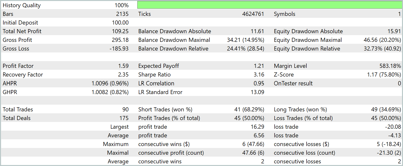
Over the four-month testing period, the initial deposit of USD 100.0 grew to USD 209.25, representing a gain of more than 109.0%. The profit factor came in at 1.59, and the overall profit-to-loss ratio was USD 295.18 to USD 185.93. A total of 90 trades were executed — half were profitable and half were unprofitable. The average profitable trade yielded USD 6.56, while the average losing trade incurred a loss of USD 4.13. On average, this generated about USD 1.21 per trade. The maximum equity drawdown was 20.2%, while the maximum balance drawdown was 14.95%.
These figures reflect not just dry statistics, but the dynamics of how the model perceives the market. Each trade was based on a careful assessment of the current market state and a forecast of key features. Linear regression of equity shows a correlation of 0.95, confirming steady capital growth. Although the standard error reflects the natural volatility and market noise that any trading system faces, the profit factor and Sharpe ratio indicate that the strategy is capable of generating risk-adjusted returns. However, the short testing period and the small number of trades call for careful attention and a cautious approach.
It is particularly interesting that the model achieves positive results not through the number of winning trades, but through the quality of each profitable trade. The average profit significantly exceeds the average loss, which makes every successful entry a foundation for capital growth. At the same time, the maximum drawdown remains moderate. A Recovery Factor of 2.35 demonstrates that, following declines, the system is able to recover quickly while maintaining control over risk.
Despite these impressive results, we are aware of the potential risks. A short testing period, a limited number of trades, and a low Z-score suggest that some of the returns may have been due to a fortunate combination of circumstances. To improve reliability, additional analysis, checks, simulations, and stress tests are required, taking into account actual costs — such as spreads, commissions, and slippage. Only after successfully passing these tests can the strategy be considered ready for live trading.
Conclusion
In this article, we completed the development and testing of an integrated model based on the BAT framework for analyzing market data and formulating a trading policy. The systematic implementation of all components — from data preparation and market state encoding to the construction of the Actor-Critic model — has resulted in a system capable of making informed trading decisions based on a comprehensive analysis of key market features.
Backtesting on historical data showed positive returns and manageable risks. The model successfully extracted meaningful signals from a chaotic stream of quotes, generating capital growth with moderate drawdowns. An analysis of the metrics confirmed that the strategy is capable of balancing risk and return, identifying profitable opportunities, and responding to changes in market conditions.
It is particularly valuable that the BAT architecture and our module integration minimize the need for manual configuration and simplify system scaling. The strategy remains transparent and amenable to analysis and refinement, and the step-by-step approach to training and testing creates a solid foundation for the model's further development.
Despite the impressive results, we emphasize the need for additional robustness tests before applying the strategy in live trading. Only systematic and careful implementation can turn successes in testing into long-term achievements in the market.
Thus, the BAT framework presented here demonstrates significant practical value for building autonomous trading systems: it combines in-depth analysis, adaptability to market conditions, and scalability, creating a reliable platform for effective trading and further research in the field of algorithmic strategies.
References
- BAT: Learning Event-Based Optical Flow with Bidirectional Adaptive Temporal Correlation
- Other articles in this series
Software used in this article
| # | Name | Type | Description |
|---|---|---|---|
| 1 | Study.mq5 | Expert Advisor | Expert Advisor for offline model training |
| 2 | StudyOnline.mq5 | Expert Advisor | Expert Advisor for online model training |
| 3 | Test.mq5 | Expert Advisor | Expert Advisor for model testing |
| 4 | Trajectory.mqh | Class library | Structure describing the system state and model architectures |
| 5 | NeuroNet.mqh | Class library | Class library for building a neural network |
| 6 | NeuroNet.cl | Library | Code library for an OpenCL program |
Translated from Russian by MetaQuotes Ltd.
Original article: https://www.mql5.com/ru/articles/20559
Warning: All rights to these materials are reserved by MetaQuotes Ltd. Copying or reprinting of these materials in whole or in part is prohibited.
This article was written by a user of the site and reflects their personal views. MetaQuotes Ltd is not responsible for the accuracy of the information presented, nor for any consequences resulting from the use of the solutions, strategies or recommendations described.



The current implementation (Study.mq5, Test.mq5, StudyOnline.mq5) usesthe names of BAT components, but architecturally does NOT IMPLEMENT the system described in the articles.
Key differences:
The encoder has been simplified — instead of a multi-layer structure (CreateFlow → MultiWindowsConv → MSRes → BiDirectCorrelation → SATMA → SpikeConvGRU2D), a single layer of `defNeuronBAT` is used.
CreateFlow is absent — there is no conversion to an event-based representation or voxel-grid formation. Data is fed in as a flat vector `HistoryBars * BarDescr`.
BiDirectCorrelation is unavailable — the bidirectional temporal correlation module is defined but not integrated into the encoder architecture.
SATMA is not used — spatially adaptive aggregation has been replaced by CrossDMHAttention (attention), which is fundamentally different.
The GRU module is missing — there is no dynamic modelling component at the motion synthesis level.
STFS is incorrectly placed — it is embedded throughout, although it was intended to be only in Study.mq5 for training.
Conclusion: the code implements a general-purpose RL trader, adapting individual ideas from BAT, but does not embody the full architecture described in the articles.
Dmitry, you have three parts to this article, each in a different version of NeuroNet.mqh... Does it matter?
Each part introduces a separate implementation block and builds on the previous ones. The full version is in the final article.
The current implementation (Study.mq5, Test.mq5, StudyOnline.mq5) usesBAT component names, but architecturally does NOT IMPLEMENT the system described in the articles.
Key differences:
The encoder has been simplified — instead of a multi-level structure (CreateFlow → MultiWindowsConv → MSRes → BiDirectCorrelation → SATMA → SpikeConvGRU2D), a single layer of `defNeuronBAT` is used.
CreateFlow is absent — there is no conversion to an event-based representation or voxel-grid formation. Data is fed in as a flat vector `HistoryBars * BarDescr`.
BiDirectCorrelation is unavailable — the bidirectional temporal correlation module is defined but not integrated into the encoder architecture.
SATMA is not used — spatially adaptive aggregation has been replaced by CrossDMHAttention (attention), which is fundamentally different.
The GRU module is missing — there is no dynamic modelling component at the motion synthesis level.
STFS is incorrectly positioned — it is embedded throughout, although it was intended to be present only in Study.mq5 for training.
Conclusion: the code implements a general-purpose RL trader, adapting individual ideas from BAT, but does not embody the full architecture described in the articles.
The `defNeuronBAT` type corresponds to the `CNeuronBAT` object , which is described at the link. It includes the specified modules.
The `defNeuronBAT` type corresponds to the `CNeuronBAT` object , which is described at the link. It includes the modules specified.
What about the high (1500+) STFS error? Do the features need normalising? I’ve tried it; the error drops dramatically… but won’t that spoil the whole idea?
I’m sorry, Dmitry. I forgot to load NeuroNet.mqh into the LLM… that’s where all the discrepancies came from.
What about the high (1500+) STFS error? Do we need to normalise the features? I’ve tried it, and the error drops dramatically… but won’t that ruin the whole idea?