Neural Networks in Trading: Bidirectional Adaptive Temporal Correlation (Main Components)
 67
 0

Introduction
The market is constantly changing — sometimes it speeds up, sometimes it comes to a standstill. At times, it produces extraneous movements that confuse less flexible models. Against this backdrop, architectures that remain robust while still detecting subtle dynamic patterns are particularly interesting to observe. BAT is one such solution. It successfully combines two elements that are rarely found together: the transparency of classical methods and the flexibility of modern approaches to sequence processing. There's no complicated math here, no computationally intensive attention mechanisms, and no huge sets of parameters. On the contrary, BAT is built around a clear transformation logic in which each step can be explained in layman's terms, without relying on engineering jargon.
The main idea behind BAT is to view a data stream as a sequence of local segments. It is as though the model divides the signal into small segments, carefully examines the behavior of each one, and then pieces together the overall picture, taking into account the contribution of all local structures. This approach is similar to that of an experienced analyst, who always examines the market from different angles before making a decision. He compares short intervals with long intervals, assesses local impulses, and pays attention to the overall trend. It is precisely this combination of local and global observations that underpins the robustness of BAT.
At the same time, the model does not just piece together parts of the signal; it can flexibly shift the emphasis. If the market exhibits a clear structure, more attention is paid to the corresponding blocks; if, however, the movement breaks down into noise, the model rationally reduces the influence of questionable sections. This adaptive behavior arises from a simple weighting mechanism that does not require complex computations but allows the model to remain stable even when dealing with turbulent data. This is a valuable quality for practical trading, where the quality of a decision is often more important than flashy architecture.
The elegance of BAT lies in its combination of lightweight design and informativeness. Despite its theoretical depth, the model does not require traders to use powerful GPUs, does not require third-party frameworks, and does not force them to overhaul their existing infrastructure. It works well in compact systems. What matters here is the model's speed, stability, and predictability. Solutions should work as precisely as a well-calibrated indicator: without delays, without unnecessary calculations, and without any uncertainty in their behavior.
In the previous article, we took an in-depth look at the structure of the BAT framework: the principle underlying its architecture and why the framework combines simplicity with flexibility. Back then, we focused more on the idea itself, viewing the architecture as a blueprint yet to be brought to life. Now, our task is to move from theory to practice.
But before we dive into the implementation, let's review the key elements of BAT. The model is based on a simple sequence of operations: transform the data, divide it into small segments, evaluate the contribution of each segment, and combine the results into a single signal. It sounds too simple, but it is precisely this straightforwardness that creates stability. Like an experienced craftsman who, before performing precise work, always starts with broad strokes, then refines the details, and finally draws a clean outline, BAT operates in a consistent, step-by-step manner, without sudden jumps or abrupt transitions. Thanks to this structured approach, it is less prone to overfitting and performs better across different market regimes.
The model begins with a preliminary data transformation. This is the very moment when raw data is carefully organized into a format suitable for further analysis. The next step is to divide the signal into local segments, which allows the model to capture the internal structure of the time series. These segments are then evaluated, and each is assigned a weight that reflects its importance. The result is a smoothed, stable representation of the signal, in which noise recedes into the background and key patterns become more prominent. This entire sequence of steps creates the balance that makes BAT easy to apply in real-world trading.
Traders often complain that modern models complicate the decision-making process, turning analysis into a struggle against confusion. With BAT, things are different. Here, even without getting into the mathematical details, it is intuitively clear why the model arrives at certain decisions. The signal strengthens where the local structure is solid and weakens where the market falters. This approach is close to traditional market reasoning, where the quality and shape of movement matter. In this sense, BAT is closer to the mindset of a professional trader than most complex neural network models.
The author's visualization of the BAT framework is shown below.
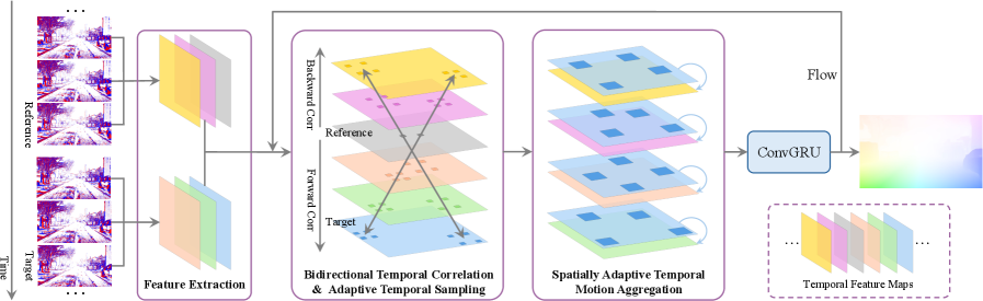
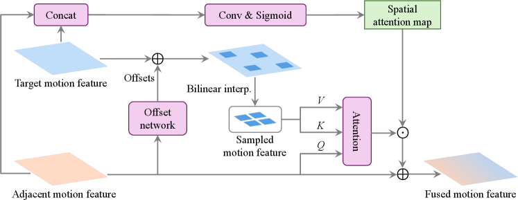
We began implementing the approaches proposed by the authors of the BAT framework at the very foundation — with the input data representation. It is important to us that the model be able to retrieve market data directly from the terminal, without any unnecessary external processing or preliminary manipulation. This allows us to maintain flexibility and make the architecture self-sufficient. After all, it is especially important for BAT to view the market as a dynamic flow that changes from moment to moment.
To adapt the price data to the logic of temporal flow, we created an event structure in which each pair of adjacent states produced a small displacement — the analogue of optical flow. In practice, it is simple: the model calculates the difference between the current and previous states, while simultaneously saving the current state for the next step. But behind this simplicity lies an important concept. We have taught the system to view the market dynamically — to sense the direction, speed, and nature of price movements, rather than simply recording static numbers.
This fundamental mechanism became the first working component of our future model. It transformed an abstract idea into a functioning pipeline already capable of processing the flow of market data, unraveling its temporal structure, and maintaining continuity in the computations.
Building on this foundation, we are moving on to the next phase of the model's development. The framework's authors emphasize that features of the dynamic flow are extracted using a six-residual-block encoder built on the principles of RAFT, which we have already had the pleasure of working with. This gives us the rare luxury of not having to design a component from scratch, but rather of carefully porting a time-tested encoder into the new architecture and integrating it into the overall processing loop. This step not only speeds up development but also builds a solid bridge between solutions that have already been tested and the challenges we will face when building the BTC module.
Bidirectional Correlation Module
The next step in our work is to build the Bidirectional Temporal Correlation (BTC) module. Here, we are essentially moving to a new level of the model, shifting from a static view of the market flow to an analysis of its internal kinematics. While in the previous step we learned how to extract stable spatial features, our task now is to identify the relationships between states over time. And not just forward, but backward as well. This will allow us to capture the signal's entire trajectory.
This module acts as a kind of market radar that detects even the slightest shifts, synchronizes movement phases, and allows the model to navigate complex price fluctuations with confidence. This is where the foundation for an accurate assessment of the dynamics is laid. Correlations link adjacent frames, reveal temporal relationships, and create a comprehensive picture of how the flow evolves.
The approach proposed by the framework's authors uses a single reference frame, then computes a series of correlations between its features and sets of frames preceding and following it in the temporal sequence. On paper, this approach looks elegant; however, when applied to our practical architecture, it immediately raises a number of questions that require careful engineering solutions.
First and foremost, we are building a system that continuously analyzes the current market situation. The model operates in real time and observes only what has already happened or is happening right now. Future data are, by definition, unavailable. Therefore, the idea of calculating correlations with frames following the reference frame is simply incompatible with the actual operation of a trading algorithm.
In addition, our step-by-step mode generates a natural state stack — a neat sequence of frames that is updated with each new time step. This stack is ideal for establishing a basis for comparison with past states: the states from one, two, or ten steps back are all readily available. Everything is built up as part of the workflow, without any additional operations. But any attempt to incorporate analogues of future frames here inevitably disrupts the logic. We cannot store what has not happened yet. And we cannot synthetically generate future states without the risk of distorting the data structure.
There is one more important detail. In our development work, we consistently strive to maximize the parallelization of computations, especially at the GPU module level, where every microsecond counts. However, the authors' proposed scheme for dividing the sequence into past and future parts results in the sequential processing of two streams and effectively doubles the computational pipeline. This not only reduces performance but also increases latency — a critical parameter for trading systems operating under real-market loads.
Therefore, when considering the original algorithm, we must look for a different approach — one that preserves its analytical power while meeting the requirements for real-time operation, data structures, and parallel execution. And in the end, our solution turns out to be much simpler and more elegant than it might seem at first glance. In order to preserve the concept of bidirectional analysis without compromising real-time requirements, we simply use — as our reference frame — not the current time step, and certainly not some hypothetical future, but rather the state located in the middle of our stack. This choice allows us to view the stream as if from a point of equilibrium: some states lie behind this point and others ahead of it within the stack's internal ordering, but all of them already exist in memory and are accessible to the model, since they arise naturally as the computational pipeline progresses.
Essentially, we temporarily freeze the center of the local window and use it as a stable reference point for calculating correlations. Half of the stack’s frames serve as historical context, smoothly reflecting recent market dynamics, while the other half consists of fresh, newly received states that have not yet become current within the main cycle but are already in the buffer. This does not violate the principles of real-time operation, since we rely exclusively on data that actually exists during execution, while fully preserving the bidirectional analysis structure of the original framework.
Thanks to this approach, we avoid artificially splitting the sequence, do not need to simulate future frames, and do not lose the ability to parallelize computations. The stack center becomes a natural counterpart to the very reference frame that the BAT authors use in their experiments. But now it is chosen to fit perfectly into a trading model with continuous data updates.
It is worth highlighting another detail at this point, one that is often left out of theoretical descriptions. The correlations generated at the output of the BTC module are not an end in themselves — they serve as input for the next stage of processing. Specifically, for MotionEncoder. And this is where an important detail comes into play. The MotionEncoder architecture is not described anywhere in the original paper by the BAT authors, leaving a gap in the information needed for practical implementation.
Instead of inventing a solution from scratch, we decided to rely on a proven approach from the TMA framework, where similar tasks had already been successfully solved. TMA's MotionEncoder is designed to accurately convert a stream of correlations into a compact, informative representation of motion while preserving local and global dependencies. This approach fits perfectly into our current pipeline: BTC generates bidirectional correlations, and MotionEncoder accurately encodes them into internal features that can then be used by other BAT modules.
In this way, we integrate a ready-made, time-tested solution into the new architecture, ensuring module compatibility and maintaining performance. This both speeds up development and provides confidence that the structure for processing the dynamic data stream remains stable and reliable.
Now that we have defined the approach to selecting a reference frame and organizing the state stack, it makes sense to show how this logic is implemented in code. In our project, it is implemented as a new object, CNeuronBiDirectCorrelation, which inherits from CNeuronTMAMFE and serves as the core of the bidirectional correlation module.
class CNeuronBiDirectCorrelation :  public CNeuronTMAMFE
  {
protected:
   CNeuronBatchNormOCL        cInpNorm;
   CNeuronBaseOCL             cRefFrame;
   CNeuronTransposeOCL        cRefFrameT;
   CNeuronMultiWindowsConvOCL cWarp;
   CNeuronBatchNormOCL        cWarpNorm;
   CNeuronBaseOCL             cCorrelation;
   CNeuronBaseOCL             cConcat;
   //---
   virtual bool      feedForward(CNeuronBaseOCL *NeuronOCL) override;
   virtual bool      calcInputGradients(CNeuronBaseOCL *NeuronOCL) override;
   virtual bool      updateInputWeights(CNeuronBaseOCL *NeuronOCL) override;

public:
                     CNeuronBiDirectCorrelation(void) {};
                    ~CNeuronBiDirectCorrelation(void) {};
   //---
   virtual bool      Init(uint numOutputs, uint myIndex, COpenCLMy *open_cl,
                          uint dimension, uint units, uint variables, uint window_out,
                          ENUM_OPTIMIZATION optimization_type, uint batch);
   //---
   virtual int       Type(void)   override const   {  return defNeuronBiDirectCorrelation;   }
   //--- methods for working with files
   virtual bool      Save(int const file_handle) override;
   virtual bool      Load(int const file_handle) override;
   virtual bool      WeightsUpdate(CNeuronBaseOCL *source, float tau) override;
   //---
   virtual void      SetOpenCL(COpenCLMy *obj) override;
  };
The object has a clear, logical internal structure in which each component has its place in the computational pipeline and is ready to operate in real time. The architecture of the internal components is defined in the initialization method.
bool CNeuronBiDirectCorrelation::Init(uint numOutputs, uint myIndex, COpenCLMy *open_cl,
                                      uint dimension, uint units, uint variables, uint window_out,
                                      ENUM_OPTIMIZATION optimization_type, uint batch)
  {
     {
      uint windows[] = {dimension, 1};
      if(!CNeuronTMAMFE::Init(numOutputs, myIndex, open_cl, units * variables, windows, window_out,
                                                                         optimization_type, batch))
         return false;
     }
First, the parent class method of the same name is called to define the neuron's basic structure, including the window size, the number of variables and outputs, and the optimization parameters.
Next, the individual blocks — which we are familiar with from previous stages of developing the algorithm — are initialized one by one. First, the input signal normalization component cInpNorm is initialized without an activation function to preserve a clean data flow.
   uint index = 0;
   if(!cInpNorm.Init(0, index, OpenCL, variables * dimension * units, iBatch, optimization))
      return false;
   cInpNorm.SetActivationFunction(None);
Next, a reference frame cRefFrame and its transposed version cRefFrameT are created, also without activation functions. This allows them to be used in correlation calculations without distortion.
   index++;
   if(!cRefFrame.Init(0, index, OpenCL, variables * dimension, optimization, iBatch))
      return false;
   cRefFrame.SetActivationFunction(None);
   index++;
   if(!cRefFrameT.Init(0, index, OpenCL, variables, dimension, optimization, iBatch))
      return false;
   cRefFrameT.SetActivationFunction(None);
The next key component — cWarp — is responsible for block convolution and the calculation of local displacements. And here it is important to highlight one subtle point. Each frame in the stack is at a different temporal distance from the reference frame, so simply comparing their features without taking this distance into account may yield results that are not entirely representative. In the original implementation of BAT, the authors assume linear motion and simply shift the frames in proportion to time.
We, on the other hand, took a more flexible approach. By using a multi-window convolution object, we allow the model to learn the displacement parameters for each state within the analyzed history window on its own. This approach makes it possible to accurately account for the unique characteristics of the dynamics of each segment of the time series, rather than relying on a predefined linear approximation. As a result, cWarp becomes a fully fledged mechanism for adaptive analysis of local displacements, capable of identifying actual relationships between market states and generating more informative features for subsequent modules.
     {
      uint windows[];
      if(ArrayResize(windows, units) < (int)units)
         return false;
      ArrayFill(windows, 0, units, dimension);
      index++;
      if(!cWarp.Init(0, index, OpenCL, windows, dimension, variables, 1, optimization, iBatch))
         return false;
      cWarp.SetActivationFunction(None);
     }
Next, cWarpNorm normalizes the convolution results, stabilizing the output and making subsequent computations more predictable.
   index++;
   if(!cWarpNorm.Init(0, index, OpenCL, cWarp.Neurons(), iBatch, optimization))
      return false;
   cWarpNorm.SetActivationFunction(None);
Finally, the cCorrelation and cConcat blocks are created. cCorrelation accumulates the calculated correlations, forming a single feature vector.
   index++;
   if(!cCorrelation.Init(0, index, OpenCL, units * variables, optimization, iBatch))
      return false;
   cCorrelation.SetActivationFunction(None);
cConcat then combines this vector with the input data for transfer to MotionEncoder, whose role is fulfilled by the parent class.
   index++;
   if(!cConcat.Init(0, index, OpenCL, (dimension + 1)*units * variables, optimization, iBatch))
      return false;
   cConcat.SetActivationFunction(None);
//---
   return true;
  }
This entire structure ensures that the object is ready for use immediately after the initialization method completes. All components are arranged in a logical order, following the data flow from input normalization through the reference frame and convolution to the final feature fusion. This not only allows for the precise implementation of the bidirectional correlation concept, but also enables the module to be effectively integrated into the overall pipeline.
The feedForward method accurately implements the forward pass logic of the bidirectional correlation module and demonstrates how the data stream is transformed step by step.
bool CNeuronBiDirectCorrelation::feedForward(CNeuronBaseOCL *NeuronOCL)
  {
   if(!cInpNorm.FeedForward(NeuronOCL))
      return false;
The algorithm begins by normalizing the input data using the cInpNorm component. At this stage, all the features under analysis are converted to a standardized scale. This is important because financial data can vary widely in amplitude: quotes for different instruments, trade volumes, or technical indicators cannot be processed as is. Normalization ensures that subsequent correlation and convolution calculations will be accurate and robust.
Next, the reference frame (cRefFrame) is selected, and its transposed version (cRefFrameT) is created. The DeConcat function is used to split the concatenated vector into segments. Specifically, the position of the reference frame in the stack (ref_position) is determined, and all preceding and subsequent states are aligned relative to it.
   uint dimension = cRefFrameT.GetWindow();
   uint variables = cRefFrameT.GetCount();
   uint units = cCorrelation.Neurons() / variables;
   uint ref_position = (units + 1) / 2;
   if(!DeConcat(cConcat.getOutput(), cRefFrame.getOutput(), cConcat.getOutput(), cInpNorm.getOutput(),
                (ref_position - 1)*dimension, dimension, (units - ref_position)*dimension, variables))
      return false;
   if(!cRefFrameT.FeedForward(cRefFrame.AsObject()))
      return false;
Next, a forward pass of the transposed reference frame is performed. This allows us to prepare the feature matrix for multiplication so that we can correctly compute local correlations with each of the neighboring frames.
The next step is to apply multi-window convolution. This is where the local displacements are calculated. The model accounts for the different temporal distance of each frame from the reference frame and learns displacement parameters for each state within the history window being analyzed.
   if(!cWarp.FeedForward(cInpNorm.AsObject()))
      return false;
This is a key difference from the original linear approximation in BAT. We allow the model to adapt to market dynamics, which improves the accuracy of feature extraction.
After convolution, the result is normalized. This stabilizes the calculations and prevents outliers from having an excessive impact, which is particularly important when dealing with financial data that exhibits sharp price movements.
   if(!cWarpNorm.FeedForward(cWarp.AsObject()))
      return false;
Next, a matrix multiplication is performed between the normalized features and the transposed reference frame. The output is a cCorrelation tensor, which captures the local correlations between the reference frame and each state in the stack.
   if(!MatMul(cWarpNorm.getOutput(), cRefFrameT.getOutput(), cCorrelation.getOutput(),
                                                units, dimension, 1, variables, true))
      return false;
This step transforms a set of individual local displacements into a single informative signal, ready for further analysis.
The next step is to concatenate the input data with the correlations. This allows the original signal to be combined with the calculated motion features, providing a comprehensive view of market dynamics for the next layer.
   if(!Concat(cInpNorm.getOutput(), cCorrelation.getOutput(), cConcat.getOutput(),
                                                 dimension, 1, units * variables))
      return false;
This approach preserves the original information while simultaneously enriching it with additional characteristics of local motion.
Finally, the combined tensor is passed to a method in the parent class, which generates motion features and integrates them into the overall BAT pipeline. This step ensures that the output of the bidirectional correlation module is correctly passed on for subsequent transformations.
Now that we have thoroughly covered the organization of a forward pass, it makes sense to move on to the next step — handling errors. Or, in other words, to the backpropagation of gradients. While the forward pass is responsible for generating features, correlations, and local displacements, the calcInputGradients method estimates each component's contribution to the model's total error and correctly distributes that error back through all layers.
bool CNeuronBiDirectCorrelation::calcInputGradients(CNeuronBaseOCL *NeuronOCL)
  {
   if(!NeuronOCL)
      return false;
First, the validity of the received pointer to the input data object is checked. If the object does not exist, the method immediately returns false. This is a standard check to ensure the validity of input data and to protect against runtime errors.
Next, the main stack parameters are defined: window size (dimension), number of variables (variables), number of elements in the sequence (units), and reference frame position (ref_position). These values are used to distribute gradients correctly throughout the state stack while maintaining consistency with the data structure built during the forward pass.
   uint dimension = cRefFrameT.GetWindow();
   uint variables = cRefFrameT.GetCount();
   uint units = cCorrelation.Neurons() / variables;
   uint ref_position = (units + 1) / 2;
In the first step, the gradients are propagated through the components of the parent class. Here, MotionEncoder performs its role: it receives the combined feature vector, encodes motion, and distributes the error across the input features.
   if(!CNeuronTMAMFE::calcInputGradients(cConcat.AsObject()))
      return false;
DeConcat is then called to split the gradients of the concatenated vector cConcat into components corresponding to the normalized input data cInpNorm and the correlations cCorrelation.
   if(!DeConcat(cInpNorm.getPrevOutput(), cCorrelation.getGradient(), cConcat.getGradient(),
                                                              dimension, 1, units * variables))
      return false;
   if(cInpNorm.Activation() != None)
      if(!DeActivation(cInpNorm.getOutput(), cInpNorm.getPrevOutput(), cInpNorm.getPrevOutput(),
                                                                         cInpNorm.Activation()))
         return false;
   Deactivation(cCorrelation)
This step mirrors the Concat operation from the forward pass, ensuring that errors are correctly propagated to each component.
If an activation function was applied at the input in cInpNorm, DeActivation is called to adjust the gradients based on the derivative of the activation function. A similar operation is performed for cCorrelation to correctly propagate the error through the linear transformations and convolution.
Next, MatMulGrad is executed to compute the gradients of the matrix multiplication between the normalized convolution features (cWarpNorm) and the transposed reference frame (cRefFrameT).
   if(!MatMulGrad(cWarpNorm.getOutput(), cWarpNorm.getGradient(),
                  cRefFrameT.getOutput(), cRefFrameT.getGradient(),
                  cCorrelation.getOutput(), units, dimension, 1, variables, true))
      return false;
   Deactivation(cWarpNorm)
   Deactivation(cRefFrameT)
The gradients are backpropagated through both objects, reflecting the influence of each element on the total error. After that, Deactivation is called for cWarpNorm and cRefFrameT to account for possible nonlinearities.
The next step is backpropagation through cWarp, where the gradients of local displacements and convolution are propagated back to the inputs.
   if(!cWarp.CalcHiddenGradients(cWarpNorm.AsObject()))
      return false;
After that, the gradients for the cInpNorm normalizer are calculated in the same way, and they are summed with the previously obtained data.
   if(!cInpNorm.CalcHiddenGradients(cWarp.AsObject()))
      return false;
   if(!SumAndNormilize(cInpNorm.getPrevOutput(), cInpNorm.getGradient(),
                       cInpNorm.getGradient(), dimension, false, 0, 0, 0, 1))
      return false;
Finally, the gradients are passed back to the input data object.
   if(!NeuronOCL.CalcHiddenGradients(cInpNorm.AsObject()))
      return false;
//---
   return true;
  }
The entire structure is designed to keep computations as parallel as possible while maintaining continuous processing of the state stack. CNeuronBiDirectCorrelation neatly implements the concept of bidirectional correlation. The reference frame is taken from the center of the stack. Past and recent states are analyzed within a single stream. At the same time, the requirement to operate in real time without accessing future data is met.
Adaptive Aggregation of Dynamics
The next stage of our work is to develop the SATMA module — a key component that will enable the model to analyze temporal dependencies in greater depth and refine its characterization of market flow dynamics. While the previous bidirectional correlation module generated local displacements and identified relationships between neighboring states, SATMA extends this idea to broader time horizons, accumulating information about market trends and structural patterns.
The primary goal of SATMA is to effectively integrate motion features and transform them into a form suitable for forecasting and subsequent use in a trading strategy. The module acts as a network-based temporal filter, identifying hidden correlations and patterns that are not apparent from local analysis of individual frames.
Architecturally, SATMA is built on an adaptive attention mechanism and multilayer transformations, which allow it to take into account both recent changes and longer-term trends. An important feature is that all operations are performed while maintaining the ability to process data in parallel, which is critical for real-time processing of market data.
As part of this project, the SATMA module has been implemented as a new object, CNeuronSATMA, which inherits from CNeuronBaseOCL and is seamlessly integrated into the overall BAT pipeline. Its structure is designed to effectively process motion features and generate an informative representation of the temporal flow.
class CNeuronSATMA  :  public CNeuronBaseOCL
  {
protected:
   CLayer                        cWarp;
   CNeuronBaseOCL                cRefFrame;
   CNeuronRelativeCrossAttention cCrossAttention;
   CNeuronConvOCL                cSpatialAttention;
   //---
   virtual bool      feedForward(CNeuronBaseOCL *NeuronOCL) override;
   virtual bool      calcInputGradients(CNeuronBaseOCL *NeuronOCL) override;
   virtual bool      updateInputWeights(CNeuronBaseOCL *NeuronOCL) override;

public:
                     CNeuronSATMA(void) {};
                    ~CNeuronSATMA(void) {};
   //---
   virtual bool      Init(uint numOutputs, uint myIndex, COpenCLMy *open_cl,
                          uint dimension, uint units, uint variables,
                          uint window_key, uint heads,
                          ENUM_OPTIMIZATION optimization_type, uint batch);
   //---
   virtual int       Type(void) override   const   {  return defNeuronSATMA; }
   //---
   virtual bool      Save(int const file_handle) override;
   virtual bool      Load(int const file_handle) override;
   //---
   virtual bool      WeightsUpdate(CNeuronBaseOCL *source, float tau) override;
   virtual void      SetOpenCL(COpenCLMy *obj) override;
   virtual void      SetActivationFunction(ENUM_ACTIVATION value)  override { };
  };
The object consists of several key components:
- cWarp is responsible for preparing local displacements and performing their initial transformation,
- cRefFrame serves as a reference frame for aligning temporal dependencies,
- cCrossAttention implements a cross-attention mechanism, allowing the module to identify the most significant temporal and spatial relationships between states.
- cSpatialAttention adds a spatial attention layer that amplifies meaningful features and suppresses noise signals, creating a clearer and more stable representation of market dynamics.
The object is initialized by carefully assembling all of the module's components step by step to ensure that both the forward pass and the backward pass function correctly.
bool CNeuronSATMA::Init(uint numOutputs, uint myIndex, COpenCLMy *open_cl,
                        uint dimension, uint units, uint variables,
                        uint window_key, uint heads,
                        ENUM_OPTIMIZATION optimization_type, uint batch)
  {
   if(!CNeuronBaseOCL::Init(numOutputs, myIndex, open_cl, dimension * units * variables,
                            optimization_type, batch))
      return false;
   activation = None;
First, the parent class method of the same name is called to set the neuron's basic parameters. The module's activation is set to None, since all transformations within SATMA are performed through normalization and attention. No separate nonlinearity at the object level is required.
Next, construction of the cWarp projection begins. First, a multi-window convolution object is created, which handles multi-layer convolution with adaptive windows
   cWarp.Clear();
   cWarp.SetOpenCL(OpenCL);
   CNeuronMultiWindowsConvOCL* mwconv = NULL;
   CNeuronBatchNormOCL*        norm = NULL;
   CNeuronBaseOCL*             neuron = NULL;
   uint index = 0;
     {
      uint windows[];
      if(ArrayResize(windows, units) < (int)units)
         return false;
      ArrayFill(windows, 0, units, dimension);
      mwconv = new CNeuronMultiWindowsConvOCL();
      if(!mwconv ||
         !mwconv.Init(0, index, OpenCL, windows, dimension, variables, 1, optimization, iBatch) ||
         !cWarp.Add(mwconv))
        {
         DeleteObj(mwconv)
         return false;
        }
      mwconv.SetActivationFunction(None);
     }
The window sizes correspond to the number of elements in the sequence being analyzed, allowing local displacements and the dynamics of each state to be taken into account effectively. After the convolution is initialized, the object is added to the dynamic array cWarp.
The next step is to add a normalizer, which stabilizes the convolution outputs, ensuring a uniform distribution of values and preventing outliers from having an excessive influence.
   index++;
   norm = new CNeuronBatchNormOCL();
   if(!norm ||
      !norm.Init(0, index, OpenCL, mwconv.Neurons(), iBatch, optimization) ||
      !cWarp.Add(norm))
     {
      DeleteObj(norm)
      return false;
     }
   norm.SetActivationFunction(None);
The normalizer is also added to cWarp and operates without an activation function.
After the projection block is prepared, a reference frame cRefFrame is created to align temporal dependencies between states.
   index++;
   if(!cRefFrame.Init(0, index, OpenCL, dimension * variables, optimization, iBatch))
      return false;
   cRefFrame.SetActivationFunction(None);
It is initialized in the standard way and has no activation function, as it is intended solely to pass features to the attention mechanism.
Next, cCrossAttention, which implements relative attention, is initialized. It links the features of each state to key positions in the window, allowing the SATMA module to identify the most significant temporal and spatial relationships between frames.
   index++;
   if(!cCrossAttention.Init(0, index, OpenCL, dimension, window_key, units * variables,
                            heads, dimension, units * variables, optimization, iBatch))
      return false;
Finally, cSpatialAttention, a spatial attention layer, is created to amplify meaningful features and suppress noise. The SIGMOID activation function is set for this object to ensure that the object's output values fall within the range [0,1].
   index++;
   if(!cSpatialAttention.Init(0, index, OpenCL, dimension, dimension, dimension, units,
                              variables, optimization, iBatch))
      return false;
   cSpatialAttention.SetActivationFunction(SIGMOID);
//---
   return true;
  }
Thus, the initialization method assembles all SATMA components step by step, carefully configuring the convolution, normalization, and attention modules.
Once initialized successfully, the object is ready to perform forward and backward passes, process the market data stream, and integrate motion features into the overall architecture.
The feedForward method implements a forward pass through the SATMA module and demonstrates how motion features extracted from the bidirectional correlation module are processed step by step.
bool CNeuronSATMA::feedForward(CNeuronBaseOCL *NeuronOCL)
  {
   CNeuronBaseOCL* prev = NeuronOCL;
   CNeuronBaseOCL* curr = NULL;
   for(int i = 0; i < cWarp.Total(); i++)
     {
      curr = cWarp[i];
      if(!curr ||
         !curr.FeedForward(prev))
         return false;
      prev = curr;
     }
First, a loop iterates over all cWarp components. At each step, the current block (curr) receives input from the previous block (prev) and performs a forward pass. Thus, local displacements and motion features are accumulated sequentially, enabling adaptive processing of the temporal window and preparing the data for the attention mechanism. After the loop completes, prev contains the final output from cWarp, ready for further processing.
Next, spatial attention is applied. It amplifies meaningful features and suppresses noise, creating a cleaner and more informative representation of market dynamics.
   if(!cSpatialAttention.FeedForward(NeuronOCL))
      return false;
The next step is to prepare the reference frame. DeConcat is used to neatly split the concatenated vector received from the previous block, extracting the features corresponding to cRefFrame.
   uint dimension = cSpatialAttention.GetWindow();
   uint units = cSpatialAttention.GetUnits();
   uint variables = cSpatialAttention.GetVariables();
   if(!DeConcat(cRefFrame.getOutput(), prev.getPrevOutput(), NeuronOCL.getOutput(),
                dimension, dimension * (units - 1), variables))
      return false;
It is important to highlight the key difference between SATMA and the bidirectional correlation module. The most recent state of the environment is used as the reference frame here, rather than the middle frame from the stack. This decision is dictated by the very nature of predictive analysis. In order to accurately assess future market movements, it is necessary to consider the dynamics of market flow specifically in relation to the current state of the market, which reflects the latest changes in prices, volume, and other market indicators. This makes it possible to generate predictive features that are as relevant as possible for analyzing short-term and medium-term movements, thereby improving forecast accuracy and the informational value of the output vector.
Next, a critically important operation is performed: the dynamics of the entire time sequence are superimposed onto the reference frame. In fact, SumVecMatrix combines accumulated features from previous states with the current market state, creating a basis for analyzing movement in the context of the latest state.
   if(!SumVecMatrix(cRefFrame.getOutput(), prev.getOutput(), prev.getOutput(), dimension, 0, 0, 0, 1))
      return false;
This allows SATMA to see not just a sequence of changes, but the dynamics relative to the current moment. This enables the model to identify current patterns, assess trends, and generate more accurate predictive features. This approach transforms the temporal stream into an informative representation, ready for subsequent analysis through the mechanism of relative attention.
After that, control is passed to cCrossAttention, which implements relative attention. It links features describing the dynamics of the analyzed states to key positions within the window, enabling SATMA to identify the most significant temporal and spatial dependencies.
   if(!cCrossAttention.FeedForward(NeuronOCL, prev.getOutput()))
      return false;
An important feature is that the attention mechanism adaptively assigns weights to states, highlighting the most informative segments of the time series.
In the final stage, the outputs of cSpatialAttention and cCrossAttention are multiplied element-wise. This operation combines local filtering with global attention information to produce a final output vector that smoothly integrates motion features for subsequent layers of the model.
   if(!ElementMult(cSpatialAttention.getOutput(), cCrossAttention.getOutput(), Output))
      return false;
//---
   return true;
  }
Thus, CNeuronSATMA seamlessly combines the preparation of local displacements, cross-attention, and a spatial filter, creating a powerful tool for analyzing temporal and spatial dependencies in market data streams. This object serves as a logical extension of the bidirectional correlation module, allowing local features to be seamlessly integrated into a more global representation of market movement.
We have put in a lot of hard work today, so we can afford to take a short break. Let the information we have covered sink in, and take a short break from thinking about new solutions. In the next article, having regained our strength and gathered fresh ideas, we will continue and bring this project to its logical conclusion.
Conclusion
The BAT framework, with our adaptations, opens up a wide range of possibilities for analyzing and forecasting market flow. Its modular architecture, which includes bidirectional correlation and SATMA, enables the effective detection of local displacements and global temporal dependencies while accumulating key motion features.
A key feature of this approach is that it integrates processing of the current market state with historical context, potentially providing high forecast accuracy and robustness to noise. The use of proven solutions, such as MotionEncoder, combined with adaptive convolution and attention mechanisms, lays the foundation for the framework's autonomous operation and accelerates computational processes.
The model generates an informative predictive representation of market dynamics, which can be integrated into algorithmic systems once final refinement and testing are complete.
References
- BAT: Learning Event-based Optical Flow with Bidirectional Adaptive Temporal Correlation
- Other articles in this series
Software used in this article
| # | Name | Type | Description |
|---|---|---|---|
| 1 | Study.mq5 | Expert Advisor | Expert Advisor for offline model training |
| 2 | StudyOnline.mq5 | Expert Advisor | Expert Advisor for online model training |
| 3 | Test.mq5 | Expert Advisor | Expert Advisor for model testing |
| 4 | Trajectory.mqh | Class library | Structure describing the system state and model architectures |
| 5 | NeuroNet.mqh | Class library | Class library for building a neural network |
| 6 | NeuroNet.cl | Library | OpenCL program code library |
Translated from Russian by MetaQuotes Ltd.
Original article: https://www.mql5.com/ru/articles/20528
Warning: All rights to these materials are reserved by MetaQuotes Ltd. Copying or reprinting of these materials in whole or in part is prohibited.
This article was written by a user of the site and reflects their personal views. MetaQuotes Ltd is not responsible for the accuracy of the information presented, nor for any consequences resulting from the use of the solutions, strategies or recommendations described.