Statistical Arbitrage Through Cointegrated Stocks (Part 8): Rolling Windows Eigenvector Comparison for Portfolio Rebalancing

Introduction

In the last article of this series, we reported a significant improvement in our statistical arbitrage strategy. The inclusion of the half-time to mean reversion in our scoring system was instrumental in addressing the extremely large average position holding time. This was the most critical flaw in our model before the inclusion of the half-time calculation in our scoring system. Its inclusion in the basket selection is, arguably, one of the factors that contributed to the promising backtest results we achieved.

The other factor was the inclusion of portfolio weights stability as a criterion in the scoring system. It helped us in filtering out baskets with potentially high oscillation in the cointegration eigenvector. Since this eigenvector is the

basis for the calculation of the spread to be traded, its stability over time has immediate consequences on the strategy's profitability.  We calculated the portfolio weights by using the In-Sample/Out-of-Sample ADF validation over the spread (IS/OOS ADF).

It is a well-known method for assessing the cointegration vector stability, and it certainly contributed to the good results we saw in the backtest. But, despite its evident robustness for research and initial validation in the scoring system, this method has some limitations.

1. For accuracy, it requires relatively long out-of-sample periods. It has low power with short out-of-sample periods, which will be the case when we need to monitor live trading.
2. It is highly sensitive to the in-sample/out-of-sample split point; that is, if we move the split point, we may have different results.
3. It doesn’t provide any insight into when or why the cointegration breaks.

As a consequence of these limitations, the IS/OOS ADF validation over the spread can perform exceptionally well in backtests, but may be misleading or even fail in live trading.

In this article, we will see how we can overcome the limitations of the IS/OOS ADF validation while extracting the maximum benefit from its strengths. We introduce the Rolling Windows Eigenvector Comparison (RWEC) for measuring the stability of the portfolio weights. The RWEC can perform well with short out-of-sample periods, is less dependent on the in-sample/out-of-sample split point, and can provide us with information about when the cointegration breaks. Getting to know when the cointegration breaks is paramount for live trading monitoring. The RWEC combined with the IS/OOS ADF method should give us a more robust assessment of the stability of the portfolio weights, not only for nice backtests, but also for the system monitoring and portfolio rebalancing on live trading.

We will see how we can take advantage of the combination of methods primarily used to evaluate the stability of the portfolio weights by using them to estimate the stability of the trading signal. We will see how we can rebalance the portfolio when the change in its weights goes beyond the expected, eventually stopping trading the basket if the cointegration breaks. We are going from the scoring system to the live trading signal monitoring. 

Stability of weights vs. stability of signal

In an ideal trader’s world, once we have found a cointegrated pair or group of stocks and their portfolio weights, things would remain the same for an indefinite time, maybe forever. But from a stat arb strategy point of view 

“the market is in a continuous state of change. That is, there is no such thing as a bullish or bearish market, candle/bar patterns, or ‘correlated stocks that play well together’. Everything is changing now and forever.”

Not only is the absolute stock price changing, but the relative price between stocks is changing. When we get the cointegration vector that defines the portfolio weights of our basket of stocks, we are taking a snapshot of the market. While it is valid and we can rely on it to assess the cointegration, to define the direction, and to set the size of our positions, it will always be a snapshot. More than that: it will always be a snapshot taken from the rearview. The cointegration vector reflects the stocks’ relative prices in the past (as any other indicator).

Now, for how long will this cointegration last? We already know that the portfolio weights are performing well on the backtests, but for how long will these portfolio weights preserve their relative values in the future? By calculating the basket’s cointegration vector, we quantified a specific mean-reversion spread to be used as a tradeable signal, but will this signal still be effective tomorrow or next week?

As frustrating as it can be, we do not have the answer to any of these questions because we cannot escape the fact that we only have the rearview as a data source. As far as we know, at the time of writing, nobody can tell for sure what the stock price will be in the next tick, let alone the relative variation of three, four, or ten stock prices simultaneously in the next days or weeks. We can only rely on probabilities.

That’s what statistical arbitrage is at its core: the use of a set of statistical tools that help us to increase the probabilities in our favor. In this specific case, it can help us to increase the probabilities of composing a basket of stocks whose cointegration vector is more likely to remain stable over time. If properly combined, the methods we have been using since the beginning of this series to test for cointegration and stationarity can help us to increase the probabilities of choosing stocks whose portfolio weights will hold on for longer. If we succeed on this task, we can say that with a certain level of confidence (90%, 95%...) our signal will still be effective tomorrow or next week.

Knowing the stability level of the cointegration vector, the portfolio weights, and the spread is not enough to move from the scoring system to live trading. We also need to estimate the signal stability. Let’s see how we can do this by better understanding the IS/OOS ADF validation we used to estimate the cointegration vector stability. Next, we will see how we can use it in tandem with the RWEC to estimate the signal stability.

IS/OOS ADF Validation

By measuring the stability of the portfolio weights and including it as a criterion for stock selection in our scoring system, we improved the quality of the top-ranked basket we used in our last backtests. You can check the full report in Part 6 of this series, where we selected the top-ranked basket without the portfolio weights stability test, and compare it with Part 7 after its inclusion in the scoring system. For a quick comparison, these are the evolution of the capital curve (Balance/Equity graph) before and after using it as a criterion.

Fig. 1. Backtest equity graph without eigenvector stability test in basket selection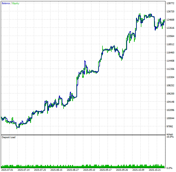

Fig. 2. Backtest equity graph with eigenvector stability test included in basket selection (previous article)

The IS/OOS ADF validation is a four-step method. It starts by splitting out our price data into two parts for in-sample (IS) and out-of-sample (OOS) tests, and computes the cointegration vector on the IS data. Then, by using this resulting cointegration vector, it calculates the spread on the OOS data and evaluates the ADF statistic on it. To consider the candidate basket’s portfolio weights as stable, both IS and OOS ADF statistics must indicate stationarity.

Split -> Estimate on IS -> Form spread on OOS -> ADF on OOS spread

As traders, we do not need to worry about the math involved, because all this magic is encapsulated for us in the professional-grade statsmodels Python library. But we must understand the process.

       n = len(prices)
        if n < 50:
            return np.nan
        split = int(n * split_ratio)
        if n - split < 30:
            return np.nan
        train = prices.iloc[:split]
        test = prices.iloc[split:]
        try:
            vec_is = self.get_coint_vector(train, method, det_order, k_ar_diff)
            spread_oos = pd.Series(np.dot(test.values, vec_is), index=test.index)
            if spread_oos.std() < 1e-10 or spread_oos.isnull().any():
                self.logger.debug("Out-of-sample spread is effectively constant or contains NaNs")
                raise ValueError("Out-of-sample spread is effectively constant or contains NaNs")
            adf_stat = adfuller(spread_oos)[0]
            return float(adf_stat)
        except Exception as e:
            self.logger.warning(f"Stability computation error: {e}")
            return np.nan

You can find the full code in the coint_ranker_auto.py script attached to the previous article.

By doing an out-of-sample validation, the IS/OOS ADF test avoids overfitting and in-sample bias. Since all of us only have past data available - the rearview we mentioned above - this is a well-known technique to simulate live trading while testing. It is the equivalent of running a forward test while backtesting in Metatrader 5 Tester.

“Forward

This option allows you to check the results of testing in order to avoid fitting to certain time intervals. During forward testing, the period set in the Date field is divided into two parts in accordance with the selected forward period (a half, one third, one fourth or a custom period when you specify the forward testing start date).The first part is the period of back testing. It is the period of Expert Advisor operation adaptation. The second part is forward testing, during which the selected parameters are checked.”

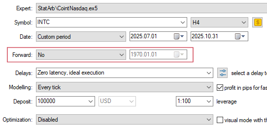
Fig. 3. Metatrader 5 Tester settings with the forward option highlithed

This OOS validation gives us a good predictive power of cointegration because it is testing the stationarity of the trading signal (the spread) “in the future”, in “unknown” data. This predictive power was reflected in the good backtest results we saw. It is saying that we can trade the calculated spread in live trading because the OOS validation has already tested it in “unknown” data. However, as all of us who run backtests know, the real question here lies in the quotes around the unknown word. How much our portfolio weights stability is guaranteed to remain stable after we leave the comfort zone of backtesting “unknown” data and go for the wild jungle of the live trading really unknown data? That is when IS/OOS ADF presents some of its weaknesses.

In live trading, we cannot wait for relatively long periods with the portfolio weights losing their stable relationship; we cannot endure long periods with a lost cointegration. We need to be informed as early as possible to make a decision and act upon it. But the IS/OOS ADF requires long out-of-sample periods for accuracy. This is not a real problem in backtesting, but it can really hurt in live trading. It happens that now these “out-of-sample periods” with potentially broken cointegration are the time our money is out there, exposed in the market, eventually causing unsustainable drawdowns.

Besides that, IS/OOS ADF is sensitive to the split point, the point in time when we split the sample data into known and “unknown” to avoid overfitting. In live trading, this split point will be moving forward continuously, so we may expect it to be less trustworthy in these conditions.

One possible solution to minimize these limitations of IS/OOS ADF for live trading is to use it with the Rolling Window Eigenvector Comparison.

Rolling Window Eigenvector Comparison

The Rolling Window Eigenvector Comparison (RWEC) calculates the portfolio weights stability by comparing the cosine distance of successive eigenvectors’ angles against a defined threshold. It computes the cointegration vector over rolling windows and compares eigenvectors across these windows.Although we are not focused on the math behind the calculation of the eigenvectors, it may be useful to remember what an eigenvector is to better understand how this method works.

“Geometrically, vectors are multi-dimensional quantities with magnitude and direction, often pictured as arrows. A linear transformation rotates, stretches, or shears the vectors upon which it acts. A linear transformation's eigenvectors are those vectors that are only stretched or shrunk, with neither rotation nor shear. The corresponding eigenvalue is the factor by which an eigenvector is stretched or shrunk. If the eigenvalue is negative, the eigenvector's direction is reversed. (Wikipedia page about Eigenvalues and Eigenvectors.)”

As traders who need to analyse this kind of data and respective plots, the relevant information is highlighted above: after the matrix linear transformation, the eigenvectors do not rotate or shear. That is, the relative angle between eigenvectors remains the same, no matter the linear transformation applied. This is the basis upon which the RWEC method is built.

The same Wikipedia page has this animation. It is the most intuitive I could find to illustrate this eigenvector’s property.

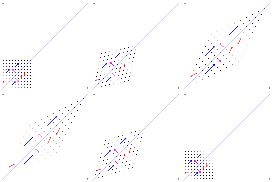
Fig. 4. Animated illustration showing that eigenvectors do not shear or rotate after a linear transformation

The magenta arrows are a representation of eigenvectors. While the other vectors, represented in blue and red, have their directions or magnitude changed by the matrix linear transformation, the magenta arrows, the eigenvectors, preserve their direction and shape. The relative angle between them, their relative inclination to each other, remains the same. 

There are other RWEC metrics that can be used to assess the stability of the cointegration vectors besides the successive eigenvectors cosine angle comparison, like the correlation of hedge ratios, but they are based on the same fundamental property of eigenvectors not changing their relative inclination after a linear transformation. (By the way, this is a fascinating field of study for those interested in deepening their understanding of this subject.)

Figures 5 and 6 show two sample plots from the RWEC method applied to two different ETF pairs over the same period. In the examples that follow, for both methods, we are using ETF pairs instead of the stock baskets we’ve been using in our experiments. The reason is that we are finishing this introduction to statistical arbitrage. We started the series with Pearson correlation for FX pairs trading and moved to stocks because they fit better to understand the process of narrowing down the market to build a sample scoring system. Now that we are going from the backtests to the live trading, we have an opportunity to return to pairs trading and leverage what we learned with the stock market: the testing methods, the building of the scoring system, and the evolution of the database. It is also the right moment to start exploring other markets and their peculiarities. To make your replication of these experiments easier, we are using only the symbols included in the Meta Quotes demo account for Metatrader 5.

The purpose of these plots is to show how clearly this method tells us the exact point in time when the stability of the portfolio weights (or the cointegration at all) was broken. This property, called high temporal resolution, is one of the main reasons that make it so useful for live trading monitoring.

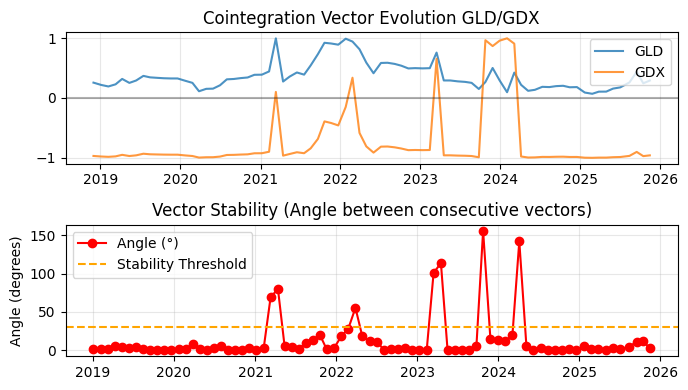
Fig. 5. Rolling Windows Eigenvector Comparison sample plot

In the first plot, the blue line represents the weight of the first asset on the pair, in this case GLD. The orange line represents the weight of its counterpart, GDX, over time. GLD is the asset we are going long; its value on the portfolio vector is positive, above the zero line. GDX is the asset to be shorted. The y-axis values are not the “real” values of the asset. They were normalized to 1 to give us the relative weight between the two assets. You can see clearly that in the beginning of 2021, 2022, and 2023, the asset to be shorted goes beyond zero, reverting its initial relationship on the pair. More than that, by the end of 2023 to the first months of 2024, they changed sides, and what should be bought now has to be sold, and vice versa. These structural market changes were reflected in their cointegration vector angles displayed in the second plot.

The red dots represent the similarity between successive cointegration vectors as a measure of the cosine distance between their respective angles, the difference between the vectors’ inclination. If this difference is zero, it means that there is no difference, that the cointegration vectors have the same inclination. When successive vectors have the same inclination, their similarity equals identity, and we have perfect stability. In this example, we only have perfect stability for brief periods. On the other hand, we have extreme peaks of imbalance, usually in the first half of the year, exactly those periods in the beginning of 2021, 202, and 2023, with an extreme peak at the beginning of 2024 when the relationship between the assets reverted.

The whole point about the RWEC method is that it measures the structural stability of the linear relationship. While the IS/OOS ADF gives us no clue about the point in time when the cointegration was lost, the RWEC shows it precisely. This feature can be used to speculate about the causes of the cointegration break: was it the result of a company merger? Perhaps one of the companies included in the pair has published a balance with exceptionally low or exceptionally high results? Maybe we had a systemic earthquake in the markets in that period? This RWEC feature may help us in finding the causes of the break in the structural stability. By knowing the causes, we can anticipate future changes of a similar nature.

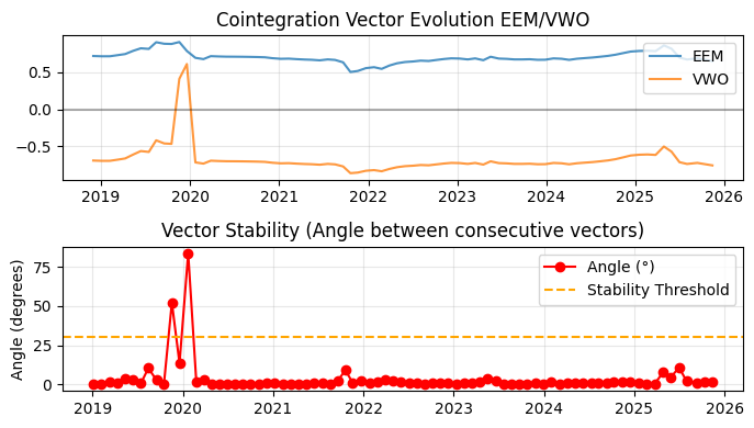
Fig. 6. Plots of a Rolling Windows Eigenvector Comparison for the EEM/VWO ETF pair

The yellow dotted line represents the chosen stability threshold. In both tests above, it was set to 30 degrees. In Figure 5, the cointegration break peak was far away from this threshold, but in Figure 6, we can see that we have a peak of nearly 80 degrees by the start of 2020. We also have two precedent deviations that were next to the 30-degree threshold. 

The RWEC stability threshold can, and should, be used as a risk management tool. Note that if we have chosen 50 degrees, the two precedent measurements would be labeled as inside the stable limit by our automated system, and the ETF pair would continue being part of our hypothetical operation. On the other hand, if we had chosen 15 degrees, the system would have recommended stopping on the second point. Since we will be using this method for monitoring live trading, this parameter choice will make our strategy more conservative if lowered, or more aggressive if the stability threshold parameter is raised.

Note that in these examples, we are using our rearview again. We know that these were peaks because we know that both pairs returned to their stable cointegration. When live trading, all that we will know is that the cointegration vector changed. We will have no means to know that it will return to its previous levels. This is when we will have to make a decision: should we stop, close eventual open positions, and leave the pair aside until it gets approved again in our scoring system, or should we change the portfolio weights to the new values?

As a trader, you probably understand that there is no hundred percent secure answer to this question. There are many factors involved in running an adaptive strategy in full automated mode. Our level of risk tolerance is the first to be taken into account. The fundamentals of each company involved in the pair/basket, the overall market dynamics, and the availability of other, better-positioned baskets in the line are all factors that we will be considering, if not systematically, intuitively, at least.

Why IS/OOS ADF and RWEC should be used together in live trading monitoring?

The short answer is: because RWEC will alert us early about the market earthquakes that IS/OOS ADF will only see later. Even when the cointegration vectors (and so the portfolio weights) remain perfectly stable, a radical change in the market may be happening underground. The IS/OOS ADF will still see the portfolio weights as the same for some time, but RWEC can alert us that something has changed. The commented tests below aim to make this RWEC property as clear as possible.

To make the IS/OOS ADF useful for live trading monitoring, we need to use Walk-Forward analysis. This way, we will have a hybrid, scoring, and monitoring framework. Instead of one IS/OOS split, we’ll be using a rolling window OOS validation, moving the split point forward by a chosen step for each test run. Note that this is the same technique used by the RWEC. The difference is that we can use IS/OOS ADF as we are doing here, or without the Walk-Forward, as we did in our scoring system.

IS/OOS ADF results

These are the results for the IS/OOS ADF for the ETF pair XLK/AAA. The horizon is 2000 bars, almost eight years, so we can have an accurate assessment of the stationarity of the spread and the cointegration vector stability.

def fetch_data(self, symbols, timeframe=mt5.TIMEFRAME_D1, n_bars=2000):

For the Walk-Forward, we set 70% of the data as the training fraction, and 100 days as the length of each out-of-sample (OOS) window. We’ve also required a Walking-Forward window of 22 trading days between the tests (the step in our range() function).

   def walk_forward_test(self, data, train_frac=0.7, oos_length=100):
        """Walk-forward OOS validation"""
        results = []
        
        n_train = int(len(data) * train_frac)
        for start in range(n_train, len(data) - oos_length, 22):  # Step = 22 trading days
            end = start + oos_length
            
            # IS: estimate cointegration
            train_data = data.iloc[:start]

You can find the full script attached here as isoos_adf_wf.py.

When running this test, you should see an output similar to this. 

IS/OOS ADF Results:

OOS Success Rate: 55.6%

Mean ADF p-value: 0.203

Median ADF p-value: 0.002

Remember that a p-value below 0.05 is our minimum acceptable to consider the spread as stationary. The p-value mean in this result is far above this minimum, indicating a non-stationary spread, while the p-value median is far below, near zero, indicating strong spread stationarity. This is not a contradiction. Instead, it is information. The difference is telling us that this mean was highly affected by outlier values. In our case, outlier values are peaks where the stationarity was lost, but the median ensures that most of the time the spread was stationary.

Last 5 windows:

adf_pvalue  stationary

4  3.111851e-01       False

5  1.517744e-01       False

6  1.718277e-03        True

7  4.409114e-07        True

8  3.135563e-05        True

The results for the last five windows indicate that the stationarity was lost around or right before the fourth OOS window.

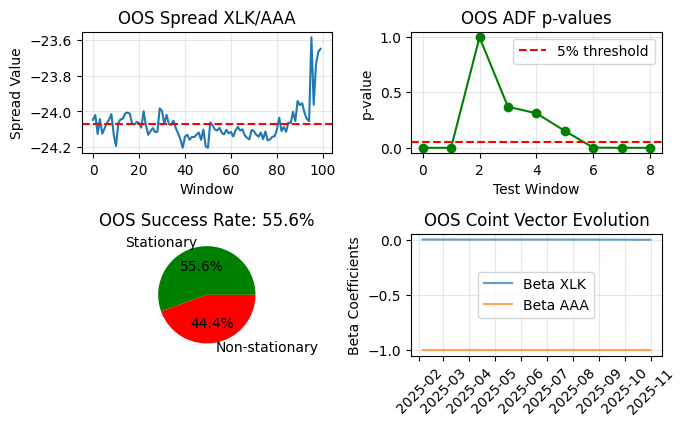
Fig. 7. Plots of a In-Sample/Out-of-Sample ADF validation for the XLK/AAA ETF pair

The four plots above show the result of the OOS Walk-Forward result in such an arrangement that one can catch the more relevant information at a glance. It is important to understand how to properly read these plots because we’ll be using them on live trading monitoring, and the overlapping windows may be a bit cumbersome if you are not familiar with their typical visualization. Let’s detail it step-by-step.

On the top-right, we have 9 data points in the x-axis with the OOS p-values. These are the same data points in the x-axis of the OOS Coint Vector Evolution plot on the bottom-right.

Remember, we have a horizon of 2000 bars? The train fraction of our test is 1400 bars (70% of 2000). So, the first in-sample run goes from day 1 through day 1400. Since we have an out-of-sample window length of 100, the first out-of-sample run goes from day 1401 to day 1500. The resulting out-of-sample p-value is our data point 0 on this plot.

We have a Walk-Forward window of 22 days, so the second in-sample test goes from day 1 through day 1422, and the second out-of-sample run goes from day 1423 to day 1522. The resulting out-of-sample p-value is our data point 1 on this plot. And so on. The very last out-of-sample run is plotted on the top-left.

As you can see, the test windows are overlapping. Thus, this is a Walk-Forward with overlapping windows. The first few p-values (0–3) are from out-of-sample periods that happened years ago (2023 to the beginning of 2025), and the last out-of-sample window closed October 31, 2025. We could have chosen a Walk-Forward without overlapping windows. Anyway you choose, it is crucial that you understand how this Walk-Forward test works, because you need to understand it so you can tweak its parameters to refine your strategy or stop trading to avoid losses.

A table may help in easing this understanding.

Walk-forward test # (x-axis in ADF plot)	In-sample period used for Beta	OOS period tested	p-value plotted	Beta plotted in bottom-right
0	Day 1 -> Day ~1400	Day 1401 -> Day 1500	Point 0	Point 0
1	Day 1 -> Day ~1422	Day 1423 -> Day 1522	Point 1	Point 1
...	...	...	...	...
8	Day 1 -> Day ~1576	Day 1577 -> Day 1677 (last 100 days)	Point 8	Point 8

Table 1. Overlapping windows in the In-Sample/Out-of-Sample ADF validation with Walk-Forward analysis

The top-left OOS Spread plot shows only the very last OOS run, the last 100-day window. That’s why it has 100 points while the ADF plot has only 9. The ADF p-value at x = 8 and the last Beta in the vector evolution plot both come from the same estimation + testing window that is shown in this plot. So we can read that this plot has a p-value of ~0.02 (well below 0.05). The spread is stationary in this last period. It is part of the green slice in the pie.

And that self-explanatory pie with the success rate is a kind of OOS stationarity fast summary. It states that from our 9 walk-forward tests, 55.6% had their stationarity confirmed.

RWEC results

These are the RWEC results for the same ETF pair, XLK/AAA. The horizon is the same 2000 bars as the IS/OOS ADF, so we can align their results by date. The Walking-Forward overlapping windows also have the same number of trading days (step=22), but the window length is different. While in the IS/OOS ADF we used oos_length=100, for the RWEC, the window=252.

   def rolling_cointegration(self, data, window=252, step=22):
        """Compute rolling cointegration vectors"""

There are two good reasons for us not to use the same 100 windows in RWEC. The first reason is technical and, in a sense, mandatory: the Johansen test author himself recommends a larger window.

“In finite samples, however, the precision of the estimates depends heavily on the sample size. Simulations show that samples of 100-200 observations (approximately 1-2 years of daily data for financial series) are often required to obtain reasonable precision of the cointegration space (...) In practice, when the parameters are not constant over time, one often applies the procedure to rolling samples of, say, 200-400 observations to check the stability of the cointegration relations.” (Johansen, 1995).

The other reason is that if at any moment we want to compare our tests with academic papers or benchmarks, it’s better that we’ve been using the recommended academic standards. By using 252 for RWEC and 100 for IS/OOS ADF, our tests are directly comparable to published research.

In practice, this difference in the window length is a direct consequence of the goals of each method. The RWEC is measuring the structural stability of the cointegration vectors. To be reliable, it needs many observations on the sample data. On the other hand, IS/OOS ADF is measuring the stationarity of the spread in the OOS data, so it must be short enough to simulate real trading. Once the technical requirements are fulfilled, it is from these practical considerations that the academic best practices emerge.

As said above, here we are using the cosine distance of the vector angles as the chosen metric for vector similarity. We set the threshold for stability as 30 degrees.

   def vector_similarity(self, vectors_df):
        """Compute cosine similarity between consecutive vectors"""
        similarities = []
        for i in range(1, len(vectors_df)):
            vec1 = vectors_df.iloc[i-1].values
            vec2 = vectors_df.iloc[i].values
            cos_sim = np.dot(vec1, vec2) / (np.linalg.norm(vec1) * np.linalg.norm(vec2))
            angle_deg = np.degrees(np.arccos(np.clip(cos_sim, -1, 1)))
            similarities.append({
                'date': vectors_df.index[i],
                'cosine_similarity': cos_sim,
                'angle_degrees': angle_deg,
                'stable': angle_deg < 30  # Threshold
            })
        return pd.DataFrame(similarities).set_index('date')

You can find the full script attached here as rwec.py.

When running this test, you should see an output similar to this. 

RWEC Results:

stable

True     29

False     4

Name: count, dtype: int64

Mean angle: 22.3°

Median angle: 0.1°

The same observations about the difference between the mean and the median angle we made above on the IS/OOS ADF results also apply here. While the mean angle is relatively near our chosen threshold, the median angle is near zero, which would be perfect stability. The cause of this difference can be easily understood in the plots below, with extreme outliers in the portfolio short side (the orange line - AAA).

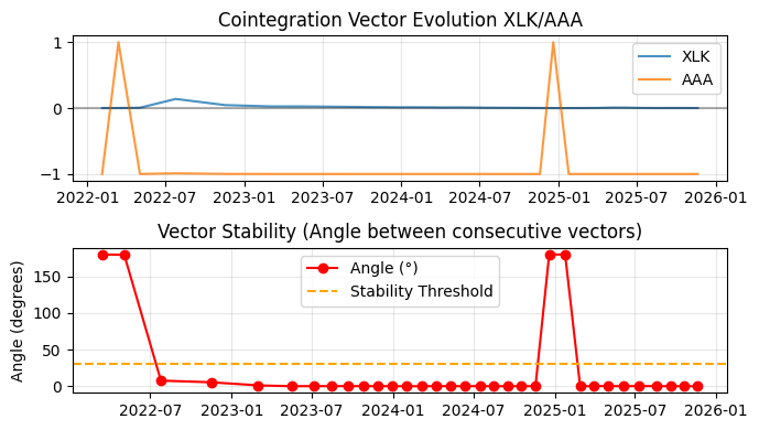
Fig. 8. Plots of a Rolling Windows Eigenvector Comparison for the XLK/AAA ETF pair

What the plots are screaming is: be cautious! This pair is stable most of the time, but it is subject to full imbalance sometimes. Note that each plot has 33 data points, 29 true/stable and 4 false/unstable (the four peaks we see in the second plot). Each instability peak took more than two months from going above our threshold to returning below it. It seems time enough to drain previous profits or even to trigger a margin call, depending on our account size. In a word, RWEC is exposing structural instability that IS/OOS ADF ignored in its last OOS window (although the 55,6% OOS success rate can be taken as an alert).

As said, I cherry-pick this ETF pair to better illustrate the point in question. From what I’ve seen, it is not so common to find such isolated high peaks of imbalance in the high-liquidity Nasdaq stocks we’ve been using as an example in this series. But it may happen, and besides that, we want our stat arb framework to be able to, at least, help us in building a stable pair or basket from any market or asset class. We do not want it to be limited to high-liquidity Nasdaq stocks.

Rebalancing interval

Once we understand how each of these tests works and how they can be used in tandem to help us in identifying unstable portfolios, the question that follows is: at which frequency should we run the analysis described above while live trading monitoring? Once a week? Twice a month? Maybe it all depends on the timeframe we are operating and we can just take a look at their plots once a day?

I ask for your permission to answer this question with the reproduction of Ed Thorp’s statistical arbitrage trading routine described by himself, as it was around 2000. Ed Thorp is a mathematician, gambler, and hedge fund manager who was among the pioneers of the quant revolution in the late 1980s. He described his trading routine in his autobiographical book “A Man for All Markets” (Random House, NY, 2017).

“The statistical arbitrage operation that Steve and I restarted in 1992 has been running successfully now for eight years. Our computers traded more than a million shares in the first hour, and we are ahead $400,000. Currently managing $340 million, we have purchased $540 million worth of stocks long and sold an equal amount short. Our computer simulations and experience show that this portfolio is close to market-neutral, which means that the fluctuations in the value of the portfolio have little correlation to the overall average price changes in the market. Our level of market neutrality, measured by what financial theorists call beta, has averaged 0.06. 

(...)

Using our model, our computers calculate daily a “fair” price for each of about one thousand of the largest, most heavily traded companies on the New York and American stock exchanges. Market professionals describe stocks with large trading volume as “liquid”; they have the advantage of being easier to trade without moving the price up or down as much in the process. The latest prices from the exchanges flow into our computers and are compared at once with the current fair value according to our model. When the actual price differs enough from the fair price, we buy the underpriced and short the overpriced. 

(...)

Scanning the computer screen, I see the day’s interesting positions, including the biggest gainers and the biggest losers. I can see quickly if any winners or losers seem unusually large. Everything looks normal. I walk down the hall to Steve Mizusawa’s office, where he is watching his Bloomberg terminal, checking for news that might have a big impact on one of the stocks we trade. When he finds events such as the unexpected announcement of a merger, takeover, spin-off, or reorganization, he tells the computer to put the stock on the restricted list: Don’t initiate a new position and close out what we have.

(...)

Our portfolio has the risk-reducing characteristics of arbitrage, but with a large number of stocks in the long side and in the short side of the portfolio, we expect the statistical behavior of a large number of favorable bets to deliver our profit. This is like card counting at blackjack again, but on a much larger scale. Our average trade size is $54,000, and we are placing a million such bets per year, or one bet every six seconds when the market is open.”

I suppose that very few of us will ever have a trading business at this scale, but the fundamental teaching is the same: don’t blink! The above describes Thorp’s daily routine, every single day. The models were checked daily for the “right fair price” of thousands of stocks. While many people think that stat arb is a kind of fire-and-forget easy money, one of the most successful hedge fund managers of all time is saying that monitoring all the time is the way to go.

This is the reason why, when it comes to live trading monitoring, I chose to bring the authoritative answer of a real-world hedge-fund manager that operates at this scale. His message is clear and pragmatic, based on real experience. Operating statistical arbitrage requires continuous monitoring. The rebalancing interval is determined by the market on a case-by-case basis.

In summary, we need to include these tests in our scoring system and, to minimize risk in a fully automated operation, we need to check them at least once a day for the active portfolio. Ideally, we need to check them at the frequency of the chosen timeframe, with the shortest possible OOS window for the IS/OOS ADF, and with sensible alerts for the periods when the RWEC cosine distance starts drifting from its median.

Conclusion

Based on the good backtest results we reported in the previous article, here we start moving the development of our statistical arbitrage framework from screening/scoring to live trading. To meet the basic requirements for live trading monitoring, we suggest the inclusion of the Walk-Forward analysis in the In-Sample/Out-of-Sample ADF validation method (IS/OOS ADF), and the introduction of the Rolling Windows Eigenvectors Comparison method (RWEC), both for the scoring system and for monitoring the portfolio weights stability while live trading.

By using a simple ETF pair as an example, we show that while ADF validation is focused on assessing continuous spread stationarity, RWEC is capable of detecting early instability of portfolio weights, becoming our primary risk control tool for live monitoring and adaptive rebalancing.

We explain the mechanics of the overlapping windows in the Walk-Forward technique and detail the readings and a possible interpretation of a sample plot of this technique on IS/OOS ADF when used in tandem with RWEC. We show that, by combining RWEC and IS/OOS ADF with Walk-Forward analysis, we can have a solid backtest and achieve dynamic risk management for live trading.

Finally, we provide sample code of the Python scripts used in the article for readers interested in experimenting with the test parameters in the same ETF pair or even other asset classes.

Filename	Description
rwec.py	Python script to run the Rolling Windows Eigenvector Comparison (RWEC) test in asset pairs with plotting.
isoos_adf_wf.py	Python script to run the In-Sample/Out-of-Sample ADF (IS/OOS ADF) validation with Walk-Forward analysis in asset pairs with plotting.
bench_runner.py	Python script to run both tests in several asset pairs simultaneously and benchmark their results.