

Feature Neutralization in MQL5: Orthogonalizing Trading Signals Against Confound Factors
 100
100
 0
0

Introduction
A trading signal that looks strong can still just be a repackaged bet on volatility or trend strength. A momentum reading grows mechanically with bigger bars, and "the market has been going up for two weeks" shows up in a plain moving-average slope for free. Feature neutralization is the check that tells the two apart: regress the raw signal on a small set of confound factors over a rolling window, and trade the residual rather than the raw value. The residual is, by construction, linearly uncorrelated with the confounds inside the window it was fitted on — what that does and does not establish about the trading sequence that follows is the subject of this article, not a detail left for the end.
This article implements the mechanism as a native MQL5 library: a rolling-window ordinary-least-squares engine with its own Gauss-Jordan solver, used by an Expert Advisor that can trade either the raw signal or the neutralized residual (a one-input switch, so the same compiled EA produces both backtests under identical settings), an indicator that plots both series, and a Python companion script that validates the solver, stress-tests it, and replays the backtest on data read either from a bundled CSV or directly from a MetaTrader 5 terminal.
The project is five files: NeutralizerEngine.mqh (the engine), FeatureNeutralizer_EA.mq5 (the Expert Advisor), FeatureNeutralizer_Ind.mq5 (the chart indicator), feature_neutralizer_companion.py (offline validation and figures), and XAUUSD_M5_2025-01-07_to_2025-01-10.csv (a fixed real-data snapshot, not required once a terminal is available — see the data-source section below). All five ship in one archive, MQL5.zip ; the Files table at the end of this article lists the path each one unpacks to.
Why a "good-looking" signal can be a mirage
A 20-bar rate-of-change momentum signal on XAUUSD M5 is mechanically larger in magnitude when the underlying is more volatile, because bigger bars produce bigger price differences over any fixed lookback — a backtest that looks strong in volatile, trending stretches and flat in quiet ones may just be tracking ATR. The same happens with trend strength: a positive momentum reading during a strong trend is partly genuine continuation and partly "the market has been going up," which a plain ADX reading already captures.
Neutralization does not add information; it removes a specific, named kind of contamination. Regressing the raw signal on a volatility proxy and a trend-slope proxy over a rolling window and keeping only the residual means: whatever those two factors could have explained about the signal, this residual does not contain. That is a narrower and more checkable claim than "found new alpha," and the rest of this article is deliberately built around that narrower claim rather than a broader one the code cannot support.
The math: rolling regression and the standardized correlation system
For a rolling window of N bars, let y be the raw signal and F the k confound factors. Centering both and dividing each factor by its own standard deviation over the window gives standardized factors Z; the fitted intercept and slopes solve the factor correlation system:
(ZᵀZ/N) g = (Zᵀyc/N)
b_k = g_k / sd(F_k)
b_0 = mean(y) - sum_k b_k * mean(F_k)
ZTZ/N is the factor correlation matrix (unit diagonal), so it is already on a fixed, known scale before any pivoting happens — that is the point of standardizing first: a pivot tolerance applied to a correlation matrix means the same thing (a share of variance inflation) regardless of whether the raw factors are priced in 0.0001 units or 100,000 units. The regression coefficients are converted back to the original factor units afterward (b_k = g_k / sd(F_k)); the residual and R² are then computed from those original-unit coefficients, so neither depends on the standardization being an internal implementation detail versus something the caller has to worry about.
The residual applied to a bar that is not in the fitted window is the neutralized signal: residual = y − (b₀ + b₁f₁ + ... + b_k f_k) . The property that this residual is uncorrelated with the factors is an in-sample one — it holds, by the normal equations, for the exact window the beta was fitted on. Applying that same beta to a bar outside the window (which is what every live and backtested trade does) does not inherit the guarantee automatically; it only holds to the extent the factor relationship is stable from one window to the next. The "Numerical correctness validation" section below checks the in-sample property directly and reports it as exactly that, and the out-of-sample decorrelation reported in the Testing section is an empirical result on this dataset, not a mathematical guarantee.
NeutralizerEngine.mqh: the rolling-window engine
CFeatureNeutralizer holds the rolling window in a circular buffer and exposes exactly the four operations an EA or indicator needs: Init() , AddObservation() , GetResidual() , and the diagnostics. FN_NUM_FACTORS fixes the factor count at compile time and sizes every array in the class; it is checked again at runtime against an EA input so a stale #define fails loudly instead of silently mis-sizing an array.
//+------------------------------------------------------------------+
//| Feature contract constants                                       |
//| Compile-time sizes and numerical tolerances of the engine.       |
//| FN_NUM_FACTORS must match the factor vector built by the caller; |
//| the tolerances are relative, so they do not depend on the units  |
//| of the signal or the factors.                                    |
//+------------------------------------------------------------------+
#define FN_NUM_FACTORS        2                   // confound factors in the regression
#define FN_MATRIX_DIM         (FN_NUM_FACTORS+1)  // fitted parameters: intercept + factors
#define FN_MIN_OBS_PER_PARAM  20                  // hard floor: observations per fitted parameter
#define FN_PIVOT_TOL          1e-8                // smallest accepted unexplained-variance fraction
#define FN_SD_REL_TOL         1e-12               // sd/|mean| below this marks a constant column
Init() also enforces a statistical floor, not just a dimensional one: it refuses a window smaller than FN_MIN_OBS_PER_PARAM (20) observations per fitted parameter. A 3-parameter fit (intercept plus 2 factors) therefore needs at least 60 bars, not the bare dimensional minimum of 4 the matrix algebra alone would allow — a window that dimensionally small would still invert, but it would fit noise, which is exactly the failure mode a width check cannot catch and a parameter-count check can.
//+------------------------------------------------------------------+
//| CFeatureNeutralizer                                              |
//| Rolling-window OLS orthogonalization engine. The signal is       |
//| regressed on the confound factors over the last N CLOSED bars;   |
//| the residual of a bar that is not in the window is the           |
//| neutralized signal. Factors and signal are centered and the      |
//| factors scaled to unit variance before the normal equations are  |
//| formed, so the solved system is the factor correlation matrix    |
//| and its tolerance does not depend on units.                      |
//+------------------------------------------------------------------+
class CFeatureNeutralizer
  {
private:
   //--- circular buffer holding the rolling window
   int      m_window;                 // rolling window length (bars)
   int      m_count;                  // observations stored so far (<= m_window)
   int      m_head;                   // next write slot in the circular buffer
   double   m_sig[];                  // signal history [m_window]
   double   m_fac[][FN_NUM_FACTORS];  // factor history [m_window][FN_NUM_FACTORS]
   //--- result of the last successful fit
   double   m_beta[FN_MATRIX_DIM];    // [0]=intercept, [1..k]=factor coefficients
   double   m_r2;                     // R-squared of the last successful fit
   bool     m_fitted;                 // true once one fit has succeeded
   int      m_failStreak;             // failed fits since the last success
   //--- k x k linear solver used by Fit()
   bool     GaussJordanSolve(double &A[][FN_NUM_FACTORS], double &b[], double &x[], const int n);
public:
   //--- lifecycle
            CFeatureNeutralizer(void);
   bool     Init(const int window);
   //--- learn: store one closed-bar observation and refit once the window is full
   bool     AddObservation(const double signal_value, const double &factors[]);
   bool     Fit(void);
   //--- score: residual of an observation that is NOT part of the window
   double   GetResidual(const double signal_value, const double &factors[]) const;
   //--- state and diagnostics
   bool     IsFitted(void)       const { return(m_fitted); }
   int      GetFailStreak(void)  const { return(m_failStreak); }
   double   GetR2(void)          const { return(m_r2); }
   double   GetBeta(const int i) const { return((i>=0 && i<FN_MATRIX_DIM) ? m_beta[i] : 0.0); }
   int      GetCount(void)       const { return(m_count); }
  };
AddObservation() stores one closed-bar observation in the circular buffer and triggers a refit once the buffer is full:
//+------------------------------------------------------------------+
//| CFeatureNeutralizer::AddObservation                              |
//| Store one CLOSED-bar observation (signal and its confound        |
//| factors) in the circular buffer and refit once the window is     |
//| full. The refit uses the new observation, so the beta it         |
//| produces may only be applied to LATER bars. Returns false on a   |
//| factor-array size mismatch or when the refit fails.              |
//+------------------------------------------------------------------+
bool CFeatureNeutralizer::AddObservation(const double signal_value, const double &factors[])
  {
   if(ArraySize(factors) != FN_NUM_FACTORS)
     {
      PrintFormat("CFeatureNeutralizer::AddObservation - expected %d factors, got %d", FN_NUM_FACTORS, ArraySize(factors));
      return(false);
     }

   m_sig[m_head] = signal_value;
   for(int k=0; k<FN_NUM_FACTORS; k++)
      m_fac[m_head][k] = factors[k];

//--- the head always points at the oldest entry once the buffer has wrapped
   m_head = (m_head + 1) % m_window;
   if(m_count < m_window)
      m_count++;

//--- a fit needs the full window; before that the engine only collects data
   if(m_count == m_window)
      return(Fit());
   return(true);
  }
Fit() does five things in order: center the signal and factors, standardize the factors, solve the correlation system, convert the solved coefficients back to the factors' original units, and compute R². A factor with (near) zero variance over the window cannot be standardized and fails the fit explicitly, rather than dividing by a near-zero number:
//+------------------------------------------------------------------+
//| CFeatureNeutralizer::Fit                                         |
//| Fit signal = b0 + b1*f1 + ... + bk*fk on the stored window. Step |
//| 1 centers the data, step 2 standardizes the factors, step 3      |
//| solves the k x k correlation system, step 4 converts the         |
//| coefficients back to the original units, step 5 computes         |
//| R-squared. On failure the previous beta is kept and the fail     |
//| streak grows, so callers can stop trading on a stale beta.       |
//+------------------------------------------------------------------+
bool CFeatureNeutralizer::Fit(void)
  {
   const int n = m_count;
   double mu[FN_NUM_FACTORS];  // factor means over the window
   double sd[FN_NUM_FACTORS];  // factor standard deviations over the window
   double ybar = 0.0;          // signal mean over the window

//--- Step 1: means of the signal and of every factor
   for(int k=0; k<FN_NUM_FACTORS; k++)
      mu[k] = 0.0;
   for(int t=0; t<n; t++)
     {
      ybar += m_sig[t];
      for(int k=0; k<FN_NUM_FACTORS; k++)
         mu[k] += m_fac[t][k];
     }
   ybar /= n;
   for(int k=0; k<FN_NUM_FACTORS; k++)
      mu[k] /= n;

//--- Step 2: standard deviations; a constant factor cannot be standardized
   for(int k=0; k<FN_NUM_FACTORS; k++)
     {
      double ss = 0.0;
      for(int t=0; t<n; t++)
        {
         double d = m_fac[t][k] - mu[k];
         ss += d*d;
        }
      sd[k] = MathSqrt(ss/n);
      if(sd[k] <= FN_SD_REL_TOL*MathAbs(mu[k]))
        {
         m_failStreak++;
         return(false);
        }
     }

//--- Step 3: correlation system (Z'Z/n) g = Z'yc/n for standardized factors Z and centered signal yc
   double A[FN_NUM_FACTORS][FN_NUM_FACTORS];
   double b[FN_NUM_FACTORS];
   double g[FN_NUM_FACTORS];
   for(int i=0; i<FN_NUM_FACTORS; i++)
     {
      b[i] = 0.0;
      for(int j=0; j<FN_NUM_FACTORS; j++)
         A[i][j] = 0.0;
     }
   for(int t=0; t<n; t++)
     {
      double z[FN_NUM_FACTORS];
      for(int k=0; k<FN_NUM_FACTORS; k++)
         z[k] = (m_fac[t][k] - mu[k])/sd[k];
      double yc = m_sig[t] - ybar;
      for(int i=0; i<FN_NUM_FACTORS; i++)
        {
         b[i] += z[i]*yc;
         for(int j=0; j<FN_NUM_FACTORS; j++)
            A[i][j] += z[i]*z[j];
        }
     }
   for(int i=0; i<FN_NUM_FACTORS; i++)
     {
      b[i] /= n;
      for(int j=0; j<FN_NUM_FACTORS; j++)
         A[i][j] /= n;
     }
   if(!GaussJordanSolve(A, b, g, FN_NUM_FACTORS))
     {
      m_failStreak++;
      return(false);  // singular: m_beta keeps its previous value
     }

//--- Step 4: back to the original units, beta0 = ybar - sum(beta_k * mu_k)
   double beta[FN_MATRIX_DIM];
   beta[0] = ybar;
   for(int k=0; k<FN_NUM_FACTORS; k++)
     {
      beta[k+1] = g[k]/sd[k];
      beta[0]  -= beta[k+1]*mu[k];
     }
   for(int i=0; i<FN_MATRIX_DIM; i++)
      m_beta[i] = beta[i];

//--- Step 5: R-squared over the fitted window; a flat signal has no variance to explain
   double ssRes = 0.0, ssTot = 0.0;
   for(int t=0; t<n; t++)
     {
      double pred = m_beta[0];
      for(int k=0; k<FN_NUM_FACTORS; k++)
         pred += m_beta[k+1]*m_fac[t][k];
      double err = m_sig[t] - pred;
      ssRes += err*err;
      ssTot += (m_sig[t] - ybar)*(m_sig[t] - ybar);
     }
   double sdY = MathSqrt(ssTot/n);
   m_r2 = (sdY > FN_SD_REL_TOL*MathAbs(ybar)) ? 1.0 - ssRes/ssTot : 0.0;

   m_failStreak = 0;
   m_fitted     = true;
   return(true);
  }
The solve itself is Gauss-Jordan elimination with partial pivoting on the correlation matrix:
//+------------------------------------------------------------------+
//| CFeatureNeutralizer::GaussJordanSolve                            |
//| Solve A x = b for the n x n system built by Fit(). A is a        |
//| correlation matrix (unit diagonal), so the pivot size is the     |
//| share of a factor's variance not explained by the factors        |
//| eliminated before it; a pivot below FN_PIVOT_TOL means a         |
//| variance inflation above 1e8 and the system is rejected. Returns |
//| false for such a system.                                         |
//+------------------------------------------------------------------+
bool CFeatureNeutralizer::GaussJordanSolve(double &A[][FN_NUM_FACTORS], double &b[], double &x[], const int n)
  {
   double aug[FN_NUM_FACTORS][FN_NUM_FACTORS+1];  // augmented matrix [A | b]
   for(int i=0; i<n; i++)
     {
      for(int j=0; j<n; j++)
         aug[i][j] = A[i][j];
      aug[i][n] = b[i];
     }

   for(int col=0; col<n; col++)
     {
      //--- partial pivoting: bring the largest remaining entry of this column to the diagonal
      int    pivotRow = col;
      double pivotVal = MathAbs(aug[col][col]);
      for(int r=col+1; r<n; r++)
         if(MathAbs(aug[r][col]) > pivotVal)
           {
            pivotVal = MathAbs(aug[r][col]);
            pivotRow = r;
           }
      if(pivotVal < FN_PIVOT_TOL)
         return(false);  // rank-deficient to tolerance
      if(pivotRow != col)
         for(int c=0; c<=n; c++)
           {
            double tmp = aug[col][c];
            aug[col][c] = aug[pivotRow][c];
            aug[pivotRow][c] = tmp;
           }

      //--- scale the pivot row so the pivot becomes 1
      double pivot = aug[col][col];
      for(int c=0; c<=n; c++)
         aug[col][c] /= pivot;

      //--- clear this column in every other row (above and below), which is what makes it Gauss-Jordan
      for(int r=0; r<n; r++)
        {
         if(r == col)
            continue;
         double f = aug[r][col];
         if(f == 0.0)
            continue;
         for(int c=0; c<=n; c++)
            aug[r][c] -= f*aug[col][c];
        }
     }

//--- the left block is now the identity, so the last column holds the solution
   for(int i=0; i<n; i++)
      x[i] = aug[i][n];
   return(true);
  }
Two numerical-stability points worth being explicit about, since both are real weaknesses of the normal-equations approach and are not fixed by pivoting alone: solving through (ZTZ)β=ZTy squares the condition number of the design relative to solving the original least-squares problem directly (e.g. via QR or SVD), so two factors that are only moderately correlated in the raw data become more strongly correlated in the squared system, and partial pivoting controls which row is used as the pivot, not the underlying conditioning of the problem being solved. Standardizing the factors before forming the correlation matrix removes the scale-dependence objection (the matrix is a correlation matrix either way, with unit diagonal, so a fixed pivot tolerance means the same thing on XAUUSD as on a pair priced three orders of magnitude smaller) but it does not remove the squared-condition-number cost itself.
For the 2-factor case used throughout this article the squaring is a second-order concern; a reader extending this to many, more-correlated factors should expect the normal-equations route to lose more precision than a QR-based solver would, and should verify that with the stress test in this article's companion script before trusting it on their own factor set.
A singular fit does not silently use default values — it keeps the previous successful beta and increments a fail counter, both exposed via the diagnostics in the next section:
//+------------------------------------------------------------------+
//| CFeatureNeutralizer::GetResidual                                 |
//| Apply the last successful beta to an observation and return      |
//| signal - fitted value. Call it BEFORE AddObservation() for the   |
//| same bar so the bar is not part of the fit that scores it.       |
//| Returns 0.0 before the first successful fit or on a factor-array |
//| size mismatch.                                                   |
//+------------------------------------------------------------------+
double CFeatureNeutralizer::GetResidual(const double signal_value, const double &factors[]) const
  {
   if(!m_fitted || ArraySize(factors) != FN_NUM_FACTORS)
      return(0.0);
   double pred = m_beta[0];
   for(int k=0; k<FN_NUM_FACTORS; k++)
      pred += m_beta[k+1]*factors[k];
   return(signal_value - pred);
  }
Keeping the previous beta on a failed fit is a trade-off stated here as one, not as an unqualified safeguard: it keeps the engine from trading on a garbage regression, but a beta that goes stale across several consecutive failed fits is itself a source of model drift — it was fitted on a window that no longer exists and may no longer describe the current relationship between the signal and the confounds. GetFailStreak() exists specifically so a caller does not have to treat "has a beta" and "has a current beta" as the same thing; the Expert Advisor section below shows it gating new entries.
FeatureNeutralizer_EA.mq5: the signal, the factors, and the bar order
The raw signal is a plain 20-bar rate of change of the close; a stand-in for whatever momentum or model-derived score a reader would actually neutralize. Two confound factors are built the same way, both with their CopyBuffer() / CopyClose() return counts checked explicitly:
//+------------------------------------------------------------------+
//| BuildRawSignal                                                   |
//| Raw momentum signal for the bar at the given shift: the rate of  |
//| change of the close over InpMomentumPeriod bars. Returns false   |
//| when either close cannot be read, so the caller skips the bar    |
//| instead of using a stale value.                                  |
//+------------------------------------------------------------------+
bool BuildRawSignal(const int shift, double &outSignal)
  {
   double closeNow[], closePast[];
   if(CopyClose(_Symbol, _Period, shift, 1, closeNow) != 1)
      return(false);
   if(CopyClose(_Symbol, _Period, shift+InpMomentumPeriod, 1, closePast) != 1)
      return(false);
   if(closePast[0] == 0.0)
      return(false);

   outSignal = (closeNow[0] - closePast[0])/closePast[0];
   return(true);
  }
//+------------------------------------------------------------------+
//| BuildFactors                                                     |
//| The two confound factors for the bar at the given shift.         |
//| factors[0] is ATR divided by the close (relative volatility);    |
//| factors[1] is the change of the moving average over              |
//| InpMASlopePeriod bars divided by the close (trend slope). Every  |
//| CopyBuffer/CopyClose return count is checked, and a short read   |
//| returns false.                                                   |
//+------------------------------------------------------------------+
bool BuildFactors(const int shift, double &factors[])
  {
   double atrBuf[], maNow[], maPast[], closeBuf[];
   if(CopyBuffer(g_atrHandle, 0, shift, 1, atrBuf) != 1)
      return(false);
   if(CopyClose(_Symbol, _Period, shift, 1, closeBuf) != 1)
      return(false);
   if(closeBuf[0] == 0.0)
      return(false);

//--- factor 0: relative volatility
   factors[0] = atrBuf[0]/closeBuf[0];

//--- factor 1: moving-average slope over InpMASlopePeriod bars, normalized by price
   if(CopyBuffer(g_maHandle, 0, shift, 1, maNow) != 1)
      return(false);
   if(CopyBuffer(g_maHandle, 0, shift+InpMASlopePeriod, 1, maPast) != 1)
      return(false);
   factors[1] = (maNow[0] - maPast[0])/closeBuf[0];
   return(true);
  }
Everything about when a bar is scored and when it is learned from comes down to one fixed rule, stated here in MQL5's own terms rather than a paraphrase of them: in this codebase, shift 1 is the last closed bar and shift 0 is the bar still forming. Every call in this project that reads market data uses shift 1 — shift 0 is never read, because a forming bar's close is not yet final. OnTick() runs once per new bar and, for the closed bar t at shift 1, does exactly two things in this order:
//+------------------------------------------------------------------+
//| OnTick                                                           |
//| Runs once per new bar. Shift 1 is the last CLOSED bar t; shift 0 |
//| is the forming bar and is never read. For bar t the order is:    |
//| score the residual against the beta fitted on bars t-N..t-1,     |
//| log, trade on that z-score, and only then add bar t to the       |
//| window, which refits the beta that will score bar t+1.           |
//+------------------------------------------------------------------+
void OnTick()
  {
   datetime formingBar = iTime(_Symbol, _Period, 0);
   if(formingBar == g_lastBarTime)
      return;  // no new bar has closed
   g_lastBarTime = formingBar;

//--- inputs of the closed bar t; skip the bar if any data call falls short
   double signal;
   double factors[FN_NUM_FACTORS];
   if(!BuildRawSignal(1, signal) || !BuildFactors(1, factors))
      return;

//--- Step 1, score: out-of-sample residual of bar t BEFORE bar t enters the window
   bool   scored   = neutralizer.IsFitted();
   double residual = 0.0;
   double resZ     = 0.0;
   if(scored)
     {
      residual = neutralizer.GetResidual(signal, factors);
      resZ     = RollingZScore(g_resHist, InpZScoreWindow, g_resCount, g_resHead, residual);
     }
   double rawZ = RollingZScore(g_rawHist, InpZScoreWindow, g_rawCount, g_rawHead, signal);

//--- Step 2, log: R-squared and fail streak written here belong to the beta that scored bar t
   LogBar(iTime(_Symbol, _Period, 1), signal, factors, scored, residual, rawZ, resZ);

//--- Step 3, trade: act on the closed-bar z-score, and only while the beta is current
   if(scored && neutralizer.GetFailStreak() <= InpMaxStaleBars)
      ManageSignals(InpTradeNeutralized ? resZ : rawZ);

//--- Step 4, learn: bar t joins the window; the refit it triggers scores bar t+1
   neutralizer.AddObservation(signal, factors);
  }
Score, then learn. The residual of bar t is computed by GetResidual() against whatever beta the engine currently holds — the beta fitted on the window ending at bar t−1, since bar t has not been added yet. Only after that call does AddObservation() add bar t to the window, and only that call can trigger a refit. So the beta that scores bar t is always the one in place before bar t was learned from, and the refit that bar t may trigger only affects the beta used to score bar t+1. This is the literal order in the code above, not a separate claim about it: the function that computes the residual runs first, the function that can change the beta runs second. "Trading the residual" means this z-scored output of GetResidual() , the EA's InpTradeNeutralized switch picks between this stream and the raw signal's, so the raw and neutralized backtests in the Testing section differ only in which z-score feeds the entry test, never in how they are logged or exited:
//+------------------------------------------------------------------+
//| Input parameters - trade logic                                   |
//| Entry threshold, protective distances, sizing and the switch     |
//| that runs the same EA on the raw signal for a like-for-like      |
//| comparison.                                                      |
//+------------------------------------------------------------------+
input group "=== Trade Logic ==="
input bool   InpTradeNeutralized = true;    // true: trade the residual z-score, false: trade the raw z-score
input double InpEntryZ           = 1.5;     // Entry threshold in standard deviations
input double InpSLATRMult        = 2.0;     // Stop-loss distance in ATR multiples
input double InpTPATRMult        = 3.0;     // Take-profit distance in ATR multiples
input double InpLotSize          = 0.10;    // Fixed lot size
input int    InpMaxStaleBars     = 3;       // Failed fits tolerated before new entries are blocked
input ulong  InpMagic            = 778001;  // Magic number
The stop distance uses the live ATR (shift 1, same as everywhere else, not the ATR baked into the factor vector the regression already consumed) so the risk distance reflects current conditions. A new entry is only taken when GetFailStreak() is at or below InpMaxStaleBars ; once the beta has failed to refresh for too many bars in a row, the EA stops opening new positions on it rather than trading an indefinitely stale regression. Every closed bar — scored or not, traded or not — is written to a CSV log, with 15 significant digits so a reader can recompute the regression from the logged inputs rather than trust the logged outputs blindly:
//+------------------------------------------------------------------+
//| RollingZScore                                                    |
//| Rolling z-score on a circular buffer of the last windowLen       |
//| values. The new value is stored first, so it is standardized     |
//| against a window that contains it and nothing later. Fewer than  |
//| 5 values or a flat window return 0.0 instead of a meaningless or |
//| exploding ratio.                                                 |
//+------------------------------------------------------------------+
double RollingZScore(double &buf[], const int windowLen, int &count, int &head, const double newValue)
  {
   buf[head] = newValue;
   head = (head + 1) % windowLen;
   if(count < windowLen)
      count++;

   double mean = 0.0;
   for(int i=0; i<count; i++)
      mean += buf[i];
   mean /= count;

   double var = 0.0;
   for(int i=0; i<count; i++)
      var += (buf[i]-mean)*(buf[i]-mean);
   var /= MathMax(count-1, 1);
   double sd = MathSqrt(var);

//--- too few values or a flat window: a deviation is not meaningful
   if(count < 5 || sd <= FN_SD_REL_TOL*MathAbs(mean))
      return(0.0);
   return((newValue-mean)/sd);
  }
//+------------------------------------------------------------------+
//| LogBar                                                           |
//| Append one row per closed bar to the CSV log in FILE_COMMON. The |
//| row holds the engine inputs (signal and factors), whether the    |
//| bar was scored, and the outputs, so the regression can be        |
//| recomputed outside MetaTrader and compared with the logged       |
//| residual. The R-squared and the fail streak belong to the beta   |
//| that scored the bar.                                             |
//+------------------------------------------------------------------+
void LogBar(const datetime barTime, const double signal, const double &factors[],
            const bool scored, const double residual, const double rawZ, const double resZ)
  {
   if(!InpWriteCSVLog || g_fileHandle == INVALID_HANDLE)
      return;
   FileWrite(g_fileHandle, TimeToString(barTime), NumToText(signal), NumToText(factors[0]), NumToText(factors[1]),
             (scored ? 1 : 0), NumToText(residual), NumToText(rawZ), NumToText(resZ),
             NumToText(neutralizer.GetR2()), neutralizer.GetFailStreak());
  }
//+------------------------------------------------------------------+
//| WriteManifest                                                    |
//| Write the feature-contract manifest to FILE_COMMON as plain      |
//| ASCII JSON. A downstream script reads factor_count from it and   |
//| refuses to analyze a log whose column count disagrees.           |
//+------------------------------------------------------------------+
void WriteManifest(void)
  {
   int h = FileOpen(InpManifestFileName, FILE_WRITE|FILE_TXT|FILE_ANSI|FILE_COMMON);
   if(h == INVALID_HANDLE)
     {
      PrintFormat("WriteManifest: cannot open %s, error %d", InpManifestFileName, GetLastError());
      return;
     }
   string json = StringFormat(
      "{\n"
      "  \"factor_count\": %d,\n"
      "  \"factors\": [\"atr_normalized_volatility\", \"ma_slope_trend\"],\n"
      "  \"lookback_window\": %d,\n"
      "  \"zscore_window\": %d,\n"
      "  \"momentum_period\": %d,\n"
      "  \"atr_period\": %d,\n"
      "  \"ma_slope_period\": %d,\n"
      "  \"max_stale_bars\": %d,\n"
      "  \"symbol\": \"%s\",\n"
      "  \"timeframe\": \"%s\"\n"
      "}\n",
      FN_NUM_FACTORS, InpLookback, InpZScoreWindow, InpMomentumPeriod, InpATRPeriod,
      InpMASlopePeriod, InpMaxStaleBars, _Symbol, EnumToString(_Period));
   FileWriteString(h, json);
   FileClose(h);
  }
//+------------------------------------------------------------------+
//| Input parameters - diagnostics                                   |
//| CSV log of every closed bar and the JSON manifest, both written  |
//| to the common data folder.                                       |
//+------------------------------------------------------------------+
input group "=== Diagnostics ==="
input bool   InpWriteCSVLog      = true;                                // Write one CSV row per closed bar
input string InpCSVFileName      = "FeatureNeutralizer_log.csv";        // CSV log file name in FILE_COMMON
input string InpManifestFileName = "FeatureNeutralizer_manifest.json";  // Manifest file name in FILE_COMMON
//+------------------------------------------------------------------+
//| OnInit                                                           |
//| Validate the feature contract and the inputs, create the         |
//| indicator handles once, allocate the z-score buffers, write the  |
//| manifest and open the CSV log. Any failure returns INIT_FAILED   |
//| so the EA never runs half-configured.                            |
//+------------------------------------------------------------------+
int OnInit()
  {
//--- the compiled engine and the intended factor set must agree
   if(InpExpectedFactorCount != FN_NUM_FACTORS)
     {
      PrintFormat("FATAL: InpExpectedFactorCount (%d) does not match FN_NUM_FACTORS (%d) in NeutralizerEngine.mqh",
                  InpExpectedFactorCount, FN_NUM_FACTORS);
      return(INIT_FAILED);
     }
   if(InpZScoreWindow < 5 || InpMaxStaleBars < 0)
     {
      Print("FATAL: InpZScoreWindow must be >= 5 and InpMaxStaleBars >= 0");
      return(INIT_FAILED);
     }
   if(!neutralizer.Init(InpLookback))
      return(INIT_FAILED);

//--- one handle per indicator for the whole run; the handles are read by BuildFactors()
   g_atrHandle = iATR(_Symbol, _Period, InpATRPeriod);
   g_maHandle  = iMA(_Symbol, _Period, InpMASlopePeriod, 0, MODE_SMA, PRICE_CLOSE);
   if(g_atrHandle == INVALID_HANDLE || g_maHandle == INVALID_HANDLE)
     {
      Print("FATAL: failed to create indicator handles");
      return(INIT_FAILED);
     }

   ArrayResize(g_rawHist, InpZScoreWindow);
   ArrayResize(g_resHist, InpZScoreWindow);
   ArrayInitialize(g_rawHist, 0.0);
   ArrayInitialize(g_resHist, 0.0);
   g_rawCount = 0;
   g_rawHead  = 0;
   g_resCount = 0;
   g_resHead  = 0;

   trade.SetExpertMagicNumber(InpMagic);
   WriteManifest();

//--- CSV keeps MQL5's default UTF-16 encoding; the Python script reads it as utf-16
   if(InpWriteCSVLog)
     {
      g_fileHandle = FileOpen(InpCSVFileName, FILE_WRITE|FILE_CSV|FILE_COMMON, ',');
      if(g_fileHandle == INVALID_HANDLE)
         PrintFormat("OnInit: cannot open %s, error %d - logging disabled", InpCSVFileName, GetLastError());
      else
         FileWrite(g_fileHandle, "bar_time", "raw_signal", "factor_vol", "factor_slope", "scored",
                   "residual", "raw_z", "residual_z", "r2", "fit_fail_streak");
     }

   g_lastBarTime = 0;
   return(INIT_SUCCEEDED);
  }
FeatureNeutralizer_Ind.mq5: watching it happen
The indicator plots the raw and neutralized z-scores in a subwindow using the same engine class as the EA, so the chart and the backtest cannot silently disagree about what the regression produced. Because the rolling window is stateful, OnCalculate() replays recent closed bars from scratch in chronological order on every new bar rather than trying to patch in only the newest one — the same score-then-learn order as the EA's OnTick() , bar by bar:
//+------------------------------------------------------------------+
//| BuildAt                                                          |
//| Raw signal and the two confound factors for the closed bar with  |
//| chronological index i, read from arrays that already hold the    |
//| whole history. Same formulas as the Expert Advisor's             |
//| BuildRawSignal() and BuildFactors(). Returns false when the bar  |
//| lacks history or a close is zero.                                |
//+------------------------------------------------------------------+
bool BuildAt(const int i, const double &close[], const double &atr[], const double &ma[],
             double &signal, double &factors[])
  {
   if(i < FirstValidBar() || close[i] == 0.0 || close[i-InpMomentumPeriod] == 0.0)
      return(false);

   signal     = (close[i] - close[i-InpMomentumPeriod])/close[i-InpMomentumPeriod];
   factors[0] = atr[i]/close[i];
   factors[1] = (ma[i] - ma[i-InpMASlopePeriod])/close[i];
   return(true);
  }
//+------------------------------------------------------------------+
//| OnCalculate                                                      |
//| Replays the most recent closed bars in chronological order on    |
//| every new bar, because the engine state depends on every         |
//| observation fed to it. For each closed bar the order is the same |
//| as in the Expert Advisor: score the residual against the current |
//| beta, then add the bar to the window. The forming bar (the last  |
//| array element) is never plotted and never fed to the engine.     |
//+------------------------------------------------------------------+
int OnCalculate(const int rates_total, const int prev_calculated, const datetime &time[],
                const double &open[], const double &high[], const double &low[], const double &close[],
                const long &tick_volume[], const long &volume[], const int &spread[])
  {
   const int first = FirstValidBar();
   if(rates_total < first + InpLookback + 5)
      return(0);  // not enough history yet
   if(prev_calculated == rates_total)
      return(rates_total);  // same bar: closed-bar values cannot change

//--- both handles must have calculated every bar before their buffers are read
   if(BarsCalculated(g_atrHandle) < rates_total || BarsCalculated(g_maHandle) < rates_total)
      return(0);
   double atr[], ma[];
   ArraySetAsSeries(atr, false);
   ArraySetAsSeries(ma, false);
   ArraySetAsSeries(close, false);
   if(CopyBuffer(g_atrHandle, 0, 0, rates_total, atr) != rates_total ||
      CopyBuffer(g_maHandle,  0, 0, rates_total, ma)  != rates_total)
      return(0);

//--- start from an empty plot, then rebuild the engine state from the oldest replayed bar
   for(int i=0; i<rates_total; i++)
     {
      BufRawZ[i] = EMPTY_VALUE;
      BufResZ[i] = EMPTY_VALUE;
     }
   if(!neutralizer.Init(InpLookback))
      return(0);

   double rawHist[], resHist[];
   ArrayResize(rawHist, InpZScoreWindow);
   ArrayResize(resHist, InpZScoreWindow);
   ArrayInitialize(rawHist, 0.0);
   ArrayInitialize(resHist, 0.0);
   int rawCount = 0, rawHead = 0, resCount = 0, resHead = 0;

   const int lastClosed = rates_total - 2;  // rates_total-1 is the forming bar
   const int start      = MathMax(first, lastClosed - InpHistoryBars + 1);
   for(int i=start; i<=lastClosed; i++)
     {
      double signal, factors[FN_NUM_FACTORS];
      if(!BuildAt(i, close, atr, ma, signal, factors))
         continue;

      //--- score first: the residual of bar i uses a beta fitted on bars before i
      BufRawZ[i] = RollingZScore(rawHist, InpZScoreWindow, rawCount, rawHead, signal);
      if(neutralizer.IsFitted())
        {
         double residual = neutralizer.GetResidual(signal, factors);
         double resZ     = RollingZScore(resHist, InpZScoreWindow, resCount, resHead, residual);
         //--- a stale beta is not plotted, matching the Expert Advisor's trading gate
         if(neutralizer.GetFailStreak() <= InpMaxStaleBars)
            BufResZ[i] = resZ;
        }

      //--- then learn: bar i joins the window and the refit scores bar i+1
      neutralizer.AddObservation(signal, factors);
     }
   return(rates_total);
  }
A residual is only plotted when the beta that produced it had a fail streak at or below the same InpMaxStaleBars gate the EA uses for new entries, so a chart reader sees the same "this beta is current" judgment the EA is actually trading on, not a residual computed from whatever beta happens to be sitting in memory.
Class API specification
| Method | Behavior |
|---|---|
| Init(window) | Allocates the circular buffers. Returns false if window is below FN_MIN_OBS_PER_PARAM × (factor count + 1). |
| AddObservation(signal, factors[]) | Stores one closed-bar observation. Triggers Fit() once the window is full, and on every call after that. |
| Fit() | Standardizes the window, solves the correlation system, converts back to original units. Returns false on a singular or badly-scaled fit; the previous beta and GetFailStreak() are unaffected except the streak increments. |
| GetResidual(signal, factors[]) | Applies the CURRENT beta to an observation not in the window. Returns 0.0 before the first successful fit. |
| IsFitted() | True once at least one fit has succeeded. Does not mean the beta is current — check GetFailStreak() for that. |
| GetFailStreak() | Consecutive failed fits since the last success. 0 means the beta in use was fitted on the most recently completed window. |
| GetR2() | R² of the last successful fit, over that fit's own window. 0.0 before any fit or if the window had ~zero signal variance. |
| GetBeta(i) | Index 0 is the intercept, 1..k are the factor coefficients, in the factors' original units. |
Numerical correctness validation
The synthetic dataset used for the first check below is built from a known, injected relationship: 1,400 bars where the raw signal is a sum of a decaying oscillatory term plus a known multiple of a volatility-like series and a trend-slope-like series plus idiosyncratic noise. Because the volatility and trend-slope exposure is injected on purpose and its coefficients are known, the before/after correlation change is checkable against ground truth rather than against an assumption:
Raw signal versus the neutralized residual, synthetic dataset
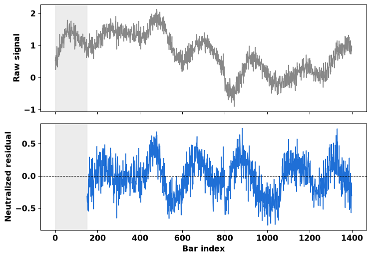
Fig. 1. Raw signal (top) and the out-of-sample neutralized residual (bottom) over the same 1,400 synthetic bars. The shaded region is the warm-up before the first fit; the residual keeps the oscillatory shape but loses the slower drift tied to the injected volatility and trend exposure.
Signal versus the volatility factor, before and after neutralization
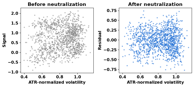
Fig. 2. Raw signal (left) and out-of-sample residual (right) plotted against the ATR-normalized volatility factor. The visible tilt on the left flattens into a shapeless cloud on the right.
Rolling R² of the fitted windows, synthetic dataset
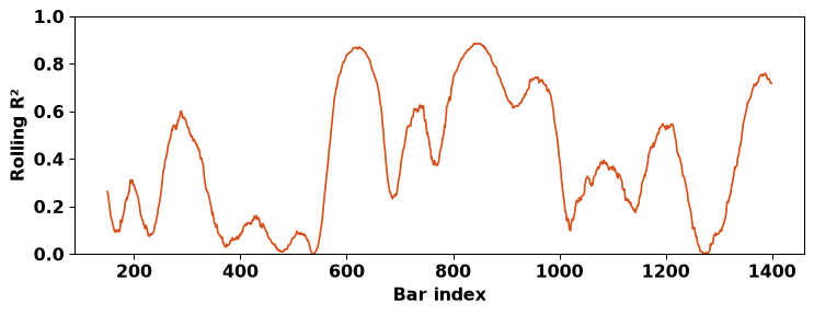
Fig. 3. R² of each window's fit over time. Stretches above 0.5 mean more than half of that window's raw-signal variance was linearly explained by the two injected confounds.
Correlation of the raw signal with the volatility factor was +0.140 before neutralization; for the out-of-sample residual — computed bar by bar against a beta that had not yet seen that bar — it falls to −0.004. The trend-slope factor moves from +0.848 to +0.101. Mean rolling R² across the fitted windows was 0.402: on average, the two injected confounds explained a little over a third of that window's raw-signal variance.
The solver itself is validated three separate ways on top of this, because agreement on one well-behaved dataset does not by itself establish robustness in general. First, the exact algorithm is mirrored in Python and checked, bar by bar on the same synthetic dataset, against numpy.linalg.lstsq solving the same standardized system via SVD — an independent numerical pathway to the same answer, not a second copy of the same elimination:
def gauss_jordan_solve(A, b, n):
    """Solve A x = b by Gauss-Jordan with partial pivoting.
    A is the factor correlation matrix (unit diagonal), so the pivot is the share
    of a factor's variance not explained by the factors eliminated before it.
    Returns (False, None) when a pivot falls below FN_PIVOT_TOL."""
    aug = [[A[i][j] for j in range(n)] + [b[i]] for i in range(n)]
    for col in range(n):
        pivot_row = col
        pivot_val = abs(aug[col][col])
        for r in range(col + 1, n):
            if abs(aug[r][col]) > pivot_val:
                pivot_val = abs(aug[r][col])
                pivot_row = r
        if pivot_val < FN_PIVOT_TOL:
            return False, None
        if pivot_row != col:
            aug[col], aug[pivot_row] = aug[pivot_row], aug[col]
        pivot = aug[col][col]
        for c in range(n + 1):
            aug[col][c] /= pivot
        for r in range(n):
            if r == col:
                continue
            f = aug[r][col]
            if f == 0.0:
                continue
            for c in range(n + 1):
                aug[r][c] -= f * aug[col][c]
    return True, [aug[i][n] for i in range(n)]
def fit_window(F, y):
    """Mirror of CFeatureNeutralizer::Fit. F is (n, k), y is (n,).
    Returns (ok, beta, r2) with beta = [intercept, b1..bk] in the original units."""
    n, k = F.shape
    mu = F.mean(axis=0)
    ybar = float(y.mean())
    sd = np.sqrt(((F - mu) ** 2).mean(axis=0))
    if np.any(sd <= FN_SD_REL_TOL * np.abs(mu)):
        return False, None, 0.0                       # a constant factor cannot be standardized
    Z = (F - mu) / sd
    yc = y - ybar
    A = (Z.T @ Z) / n                                 # correlation matrix
    b = (Z.T @ yc) / n
    ok, g = gauss_jordan_solve(A.tolist(), b.tolist(), k)
    if not ok:
        return False, None, 0.0
    beta = np.empty(k + 1)
    beta[0] = ybar
    for j in range(k):
        beta[j + 1] = g[j] / sd[j]
        beta[0] -= beta[j + 1] * mu[j]
    pred = beta[0] + F @ beta[1:]
    ss_res = float(((y - pred) ** 2).sum())
    ss_tot = float(((y - ybar) ** 2).sum())
    sd_y = math.sqrt(ss_tot / n)
    r2 = 1.0 - ss_res / ss_tot if sd_y > FN_SD_REL_TOL * abs(ybar) else 0.0
    return True, beta, r2
def run_engine_mirror(raw, factors, window, first=0):
    """Replay the EA order on every bar: score bar t with the beta fitted on the bars
    before t, THEN add bar t to the window. Returns residual, r2, fail streak, scored."""
    n = len(raw)
    res = np.full(n, np.nan)
    r2 = np.full(n, np.nan)
    streak = np.zeros(n, dtype=int)
    scored = np.zeros(n, dtype=bool)
    eng = EngineMirror(window, factors.shape[1])
    for i in range(first, n):
        if np.isnan(raw[i]) or np.any(np.isnan(factors[i])):
            continue
        if eng.fitted:                                # step 1: score (bar i is not in the window yet)
            res[i] = eng.residual(raw[i], factors[i])
            r2[i] = eng.r2
            streak[i] = eng.fail
            scored[i] = True
        eng.add(raw[i], factors[i])                   # step 2: learn
    return res, r2, streak, scored
| Metric | Result |
|---|---|
| Windows compared | 1,250 (of 1,400 synthetic bars) |
| Max |residual difference| | 3.830 × 10⁻¹⁵ |
| Mean |residual difference| | 7.279 × 10⁻¹⁶ |
| Max |R² difference| | 4.441 × 10⁻¹⁶ |
| Worst in-sample |corr(residual, factor)| over 200 sampled windows | 2.67 × 10⁻¹⁵ |
The last row is the in-sample orthogonality property stated precisely in the Math section: a fitted window's own residual is checked directly against its own factors, not against the next window's. Second, the same comparison is repeated under conditions the first run does not cover: factor scales from 10-8 to 106 and factor correlations up to 1−10-9, 200 random draws per case, against lstsq solving the standardized design (the fair reference, since it has no scale problem of its own to confound the comparison) — and, for contrast, a simpler alternative: normal equations on the raw (unstandardized) design with an absolute 1e-10 pivot threshold, which is the natural first thing to try and exactly where the scale-dependence weakness described above actually shows up numerically:
def stress_table(draws=200, n=150, seed=11):
    """Worst-case |residual difference| for badly scaled and nearly collinear factors.
    Reference: numpy.linalg.lstsq on the column-standardized design (a different solver, SVD,
    on a design that has no scale problem of its own). Compared: the engine, the legacy raw
    normal equations with an absolute pivot threshold, and plain lstsq on the unscaled design."""
    rng = np.random.default_rng(seed)
    cases = [("scale 1, rho 0.3", 1, 1, 0.3), ("scale 1e-4, rho 0.3", 1e-4, 1e-4, 0.3),
             ("scale 1e-8, rho 0.3", 1e-8, 1e-8, 0.3), ("scale 1e6, rho 0.3", 1e6, 1e6, 0.3),
             ("scales 1e-8 and 1e6, rho 0.3", 1e-8, 1e6, 0.3), ("scale 1, rho 0.999", 1, 1, 0.999),
             ("scale 1, rho 0.999999", 1, 1, 0.999999), ("scale 1, rho 1-1e-9", 1, 1, 1 - 1e-9),
             ("scale 1, duplicate factor", 1, 1, 1.0)]
    out = []
    for name, s1, s2, rho in cases:
        ok_e = ok_l = 0
        worst_e = worst_l = worst_p = 0.0
        for _ in range(draws):
            z1 = rng.standard_normal(n + 1)
            z2 = rho * z1 + math.sqrt(max(1 - rho * rho, 0.0)) * rng.standard_normal(n + 1)
            F = np.column_stack([4 * s1 + s1 * z1, 4 * s2 + s2 * z2])
            y = 0.3 + 0.8 * z1 - 0.5 * z2 + 0.5 * rng.standard_normal(n + 1)
            Xf, yf, x_new, y_new = F[:n], y[:n], F[n], y[n]
            mu, sd = Xf.mean(axis=0), Xf.std(axis=0)
            Zf = np.column_stack([np.ones(n), (Xf - mu) / sd])
            b_ref, *_ = np.linalg.lstsq(Zf, yf, rcond=None)
            res_ref = y_new - float(np.concatenate([[1.0], (x_new - mu) / sd]) @ b_ref)
            b_plain, *_ = np.linalg.lstsq(np.column_stack([np.ones(n), Xf]), yf, rcond=None)
            res_plain = y_new - float(np.concatenate([[1.0], x_new]) @ b_plain)
            worst_p = max(worst_p, abs(res_plain - res_ref))
            ok, beta, _ = fit_window(Xf, yf)
            if ok:
                ok_e += 1
                worst_e = max(worst_e, abs((y_new - (beta[0] + beta[1:] @ x_new)) - res_ref))
            okl, bl = legacy_raw_normal_equations(Xf, yf)
            if okl:
                ok_l += 1
                worst_l = max(worst_l, abs((y_new - float(np.concatenate([[1.0], x_new]) @ bl)) - res_ref))
        out.append((name, ok_e / draws, worst_e if ok_e else float("nan"),
                    ok_l / draws, worst_l if ok_l else float("nan"), worst_p))
return out | Case (200 draws each) | Engine: fit rate | Engine: worst |Δresidual| vs lstsq | Raw normal eqns: fit rate | Raw normal eqns: worst result |
|---|---|---|---|---|
| scale 1, correlation 0.3 | 1.00 | 2.4e-15 | 1.00 | 7.2e-14 |
| scale 10-4, correlation 0.3 | 1.00 | 2.0e-15 | 1.00 | 5.0e-14 |
| scale 10-8, correlation 0.3 | 1.00 | 5.3e-15 | 0.00 | singular (1e-10 abs. threshold) |
| scale 106, correlation 0.3 | 1.00 | 2.2e-15 | 1.00 | 5.1e-14 |
| scales 10-8 and 106 mixed | 1.00 | 2.2e-15 | 1.00 | 5.0e-14 |
| scale 1, correlation 0.999 | 1.00 | 1.5e-13 | 1.00 | 2.5e-12 |
| scale 1, correlation 0.999999 | 1.00 | 2.2e-10 | 1.00 | 2.2e-09 |
| scale 1, correlation 1−10-9 (near-duplicate) | 0.00 | correctly refused | 1.00 | 1.8e-06 (accepted, less accurate) |
| scale 1, exact duplicate factor | 0.00 | correctly refused | 0.00 | correctly refused |
Three results worth stating plainly rather than summarizing away. The scale-mixed case (10-8 next to 106) is where the raw, unstandardized normal equations accept a fit and get a visibly wrong answer (worst difference 2.49, not a rounding-sized number) while still reporting success — a concrete demonstration of the scale-dependence weakness an absolute pivot threshold on an unstandardized design has in general, and exactly what standardizing the factors before forming the correlation matrix fixes: the engine used in this article stays accurate to 2.2×10⁻¹⁵ on that same case.
Second, near-exact collinearity (correlation 1−10-9) is where the current engine is stricter than the raw approach, not more permissive: it refuses the fit outright (correctly, since that system is not distinguishable from singular at double precision) where the raw approach still returns a number, just a less accurate one (1.8×10⁻⁶ off). Third, neither approach, nor the numpy reference they are both checked against, is evidence of robustness on data this stress test does not cover — real confound factors with fat-tailed, non-Gaussian or regime-switching structure, for instance. The honest scope of this validation is: the algorithm matches an independent solver on everything tested here, across nine deliberately adversarial scale/correlation combinations, not on every input a factor set could ever produce.
Separately, and stated here because it bears directly on what "the solver is correct" can mean: this specific validation run checked the Python mirror of the algorithm against numpy, not the compiled .mqh itself running inside a MetaTrader 5 terminal — those are two different binaries, and agreement between the Python mirror and numpy does not by itself prove the compiled MQL5 file produces the same numbers. The --ea-log option described next exists specifically to close that gap: it checks the actual compiled EA's own logged output, not a second copy of the algorithm.
Third, and specific to the gap just named: the companion script can recompute the regression directly from a CSV log written by the compiled EA and compare the recomputed residual and R² against what the EA itself logged — checking the actual running binary, not only the algorithm as mirrored in Python:
def compare_with_ea_log(log_path, window=None):
    """Recompute the regression from the inputs the compiled EA logged and compare it with the
    residual and R-squared the EA logged. The log is MQL5's default UTF-16 CSV; the manifest
    next to it is ASCII JSON and must agree with the number of factor columns."""
    manifest_path = os.path.join(os.path.dirname(log_path), "FeatureNeutralizer_manifest.json")
    manifest = None
    if os.path.exists(manifest_path):
        with open(manifest_path, encoding="utf-8") as f:
            manifest = json.load(f)
    with open(log_path, encoding="utf-16", newline="") as f:
        rows = list(csv.DictReader(f))
    fcols = [c for c in rows[0].keys() if c.startswith("factor_")]
    if manifest is not None and manifest["factor_count"] != len(fcols):
        raise SystemExit("manifest factor_count %d != %d factor columns in the log"
                         % (manifest["factor_count"], len(fcols)))
    if window is None:
        window = manifest["lookback_window"] if manifest else 150
    raw = np.array([float(r["raw_signal"]) for r in rows])
    F = np.array([[float(r[c]) for c in fcols] for r in rows])
    ea_res = np.array([float(r["residual"]) for r in rows])
    ea_r2 = np.array([float(r["r2"]) for r in rows])
    ea_scored = np.array([int(r["scored"]) for r in rows], dtype=bool)
    ea_streak = np.array([int(r["fit_fail_streak"]) for r in rows])
    res, r2, streak, scored = run_engine_mirror(raw, F, window)
    if not np.array_equal(scored, ea_scored):
        print("scored flags differ in %d rows" % int((scored != ea_scored).sum()))
    m = scored & ea_scored & (streak == 0) & (ea_streak == 0)
    print("rows compared: %d" % int(m.sum()))
    print("max |residual difference| = %.3e" % np.max(np.abs(res[m] - ea_res[m])))
    print("max |R2 difference|       = %.3e" % np.max(np.abs(r2[m] - ea_r2[m])))
Run against a log generated from the Python mirror itself as a smoke test of the comparison tool: 350 rows compared (rows where both sides reported a fresh fit), max residual difference 8.2×10⁻¹⁵, max R² difference 2.3×10⁻¹⁵. Against a log from the actual compiled EA this becomes the real cross-check; a mismatch above floating-point noise there would point at a real divergence between the MQL5 and Python implementations, not at this script's own arithmetic.
The edge cases the engine is built to catch, exercised directly through the same Python mirror:
| Case | Observed behavior |
|---|---|
| Singular design (two identical factor columns) | Fit() refuses; previous beta kept, fail streak increments. |
| Well-conditioned control fit | Fit() succeeds; beta and R² match the generating coefficients within sampling noise. |
| Constant factor column | Refused at the standardization step (sd ≤ FN_SD_REL_TOL × |mean|), before the solve is attempted. |
| Zero-variance signal window | Fit() still solves the system; R² is explicitly set to 0.0 rather than dividing by a near-zero sum of squares. |
| Flat window for RollingZScore() | Returns 0.0 rather than dividing by a near-zero standard deviation. |
| Window below the statistical floor | Init() rejects it with the exact floor value named in the error. |
| 90 of 150 required observations | IsFitted() stays false; no residual, no trade, no plotted value. |
| Fail streak on a run of singular windows | Fitted stays false and the streak counts every failure, so GetFailStreak() reflects reality rather than resetting on a non-fit. |
Getting real market data: MetaTrader 5 or the bundled CSV
The companion script can read OHLC history directly from a running MetaTrader 5 terminal through the MetaTrader5 Python package — any symbol, timeframe, bar count, or explicit date range the terminal has, which is what makes a reader's own re-run genuinely reproducible against their own broker history rather than tied to one fixed snapshot:
def load_ohlc_mt5(symbol, timeframe, bars=5000, date_from=None, date_to=None):
    """Read closed bars from a running MetaTrader 5 terminal (MetaTrader5 package).
    Bar-count mode starts at position 1, which skips the forming bar."""
    import MetaTrader5 as mt5                          # imported here so --source csv needs no terminal
    tf = getattr(mt5, "TIMEFRAME_" + timeframe.upper(), None)
    if tf is None:
        raise ValueError("unknown timeframe " + timeframe)
    if not mt5.initialize():
        raise RuntimeError("MT5 initialization failed: %s" % (mt5.last_error(),))
    try:
        if not mt5.symbol_select(symbol, True):
            raise RuntimeError("symbol %s is not available: %s" % (symbol, mt5.last_error()))
        if date_from is not None and date_to is not None:
            rates = mt5.copy_rates_range(symbol, tf, date_from, date_to)
        else:
            rates = mt5.copy_rates_from_pos(symbol, tf, 1, bars)
    finally:
        mt5.shutdown()
    if rates is None or len(rates) == 0:
        raise RuntimeError("the terminal returned no bars for %s %s" % (symbol, timeframe))
    t = [datetime.fromtimestamp(int(r), tz=timezone.utc).strftime("%m/%d/%Y %H:%M") for r in rates["time"]]
    return (t, np.asarray(rates["open"], float), np.asarray(rates["high"], float),
            np.asarray(rates["low"], float), np.asarray(rates["close"], float))
def load_ohlc(args): """Choose the OHLC source. Returns (t, o, h, l, c, description).""" date_from = date_to = None if args.date_from and args.date_to: date_from = parse_datetime_arg(args.date_from) date_to = parse_datetime_arg(args.date_to) if args.source in ("mt5", "auto"): try: t, o, h, l, c = load_ohlc_mt5(args.symbol, args.timeframe, args.bars, date_from, date_to) return t, o, h, l, c, "MetaTrader 5 terminal: %s %s, %d bars" % (args.symbol, args.timeframe, len(c)) except Exception as exc: # ImportError, no terminal, no symbol if args.source == "mt5": raise print("[MetaTrader 5 not available (%s) - using the bundled CSV]" % exc) path = find_fallback_csv(args.csv) t, o, h, l, c = load_ohlc_csv(path) return t, o, h, l, c, "bundled CSV %s: %d bars" % (os.path.basename(path), len(c))
The default is --source auto : use a running terminal via the MetaTrader 5 package when one is available, fall back to the bundled XAUUSD_M5_2025-01-07_to_2025-01-10.csv (713 real XAUUSD M5 bars, a third-party retail feed, not broker-certified) when it is not. A terminal is not always open at the moment someone is reading or re-running this script, and the point of a fallback is that the figures and tables stay reproducible either way — without it, anyone without MetaTrader 5 running at that exact moment would get no output at all rather than a result they can compare against the article. --source mt5 forces the terminal path and raises an error instead of falling back, for a reader who wants certainty about where the numbers came from.
The Testing section below uses that forced path: every number and figure there was produced on a real MetaTrader 5 terminal, over a UTC window chosen to match the bundled CSV's own 2025-01-07 09:40 to 2025-01-10 00:00 span (the file name states that exact span, since a vague "sample" name would say nothing about which 713 bars it actually holds) —
python feature_neutralizer_companion.py --source mt5 --symbol XAUUSD --timeframe M5 --date-from "2025-01-07 09:40" --date-to "2025-01-10 00:00"
— which returned 719 bars spanning 2025-01-07 09:40 to 2025-01-09 23:50, not the CSV's 713 bars to 2025-01-10 00:00. The two don't match exactly because the CSV's feed and a live broker's server time are not guaranteed to agree to the minute; this is the expected outcome of asking two different data sources for "the same" window, not a bug in either one. A reader can reproduce a longer, broker-verified history with --source mt5 --symbol XAUUSD --timeframe M5 --bars 20000 , or any other window with --date-from / --date-to .
Testing: a real-data bar-replay comparison
This is a Python bar-by-bar replay of the EA's own order (score, then learn) on real OHLC data, run twice with the entry signal swapped — identical window, identical z-score settings, identical SL/TP, identical starting bar for both runs:
def bar_replay_backtest(h, l, c, atr, z, entry_z, sl_mult, tp_mult, start_idx, tradable):
    """One position at a time. The z-score of the closed bar i opens a trade at c[i]
    (a stand-in for the next bar's open); SL and TP are ATR multiples of bar i. Exits are
    checked from bar i+1 on; when one bar's range touches both levels the stop is assumed to
    trigger first. Returns trades (points and R multiples) and the cumulative P&L per bar."""
    n = len(c)
    trades, equity = [], [0.0]
    in_pos, side, entry, sl, tp, entry_atr = False, 0, 0.0, 0.0, 0.0, 0.0
    for i in range(start_idx, n):
        if in_pos:
            hit_sl = (side == 1 and l[i] <= sl) or (side == -1 and h[i] >= sl)
            hit_tp = (side == 1 and h[i] >= tp) or (side == -1 and l[i] <= tp)
            if hit_sl or hit_tp:
                exit_price = sl if hit_sl else tp
                pnl = (exit_price - entry) * side
                trades.append({"pnl_points": pnl, "r_multiple": pnl / (sl_mult * entry_atr)})
                equity.append(equity[-1] + pnl)
                in_pos = False
                continue
        elif tradable[i] and not np.isnan(z[i]) and abs(z[i]) > entry_z:
            side = 1 if z[i] > 0 else -1
            entry, entry_atr = c[i], atr[i]
            sl = entry - side * sl_mult * entry_atr
            tp = entry + side * tp_mult * entry_atr
            in_pos = True
        equity.append(equity[-1])
    return trades, equity
It is explicitly not a Strategy Tester run, and the gap is concrete rather than a disclaimer: no spread, no commission, no slippage, no broker execution model; when a single bar's range would touch both the stop and the target, this replay assumes the stop triggers first, which is the conservative assumption and not a verified fact about what price path actually occurred inside that bar; and P&L is reported in raw price points, which does not translate into account currency without the instrument's actual contract specification from a broker. None of that is fixable from outside MetaTrader — it is why this section is a mechanism check, not a profitability claim.
Real-data bar-replay backtest, raw signal vs. neutralized residual
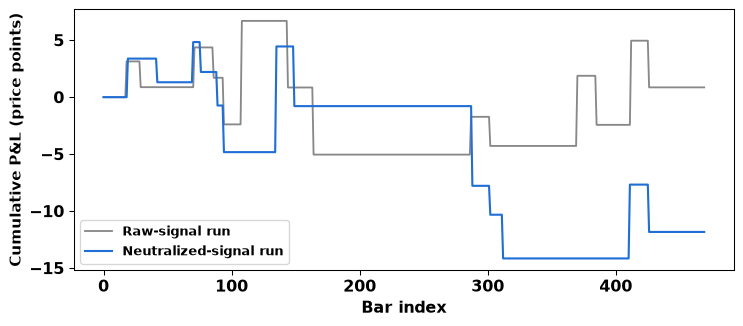
Fig. 4. Cumulative P&L in price points, 719 real XAUUSD M5 bars pulled from a live MetaTrader 5 terminal, 2025-01-07 09:40 to 2025-01-09 23:50: raw-signal run (grey) vs. neutralized-signal run (blue), identical settings for both.
| Metric | Raw signal | Neutralized residual |
|---|---|---|
| Trades | 14 | 13 |
| Net profit (points) | 0.86 | -11.83 |
| Profit factor | 1.03 | 0.66 |
| Expected payoff (pts/trade) | 0.062 | -0.910 |
| Max drawdown (points) | 11.74 | 18.99 |
| Sharpe (per trade) | 0.21 | -0.69 |
The same deterministic warm-up as the synthetic dataset — factor history needs 100 bars, then the 150-bar window needs to fill — puts the first scored bar at index 250, so 469 of the 719 bars were scored. Correlation of the raw signal with the two factors over those bars was −0.050 (volatility) and −0.260 (trend slope); for the out-of-sample residual — the actual series traded, computed bar by bar against the beta in place before each bar, never a beta that had already seen it — the trend-slope correlation falls to −0.117, roughly in line with what the regression is meant to do, but the volatility correlation moves to −0.130, larger in magnitude than it started. The mean R² of the fits used for scoring was 0.214.
That volatility result is worth stating plainly rather than explaining away, because it is exactly the failure mode named in the Limitations section below: out-of-sample decorrelation is not guaranteed by the math, only the in-sample property is, and here is a real window where one of the two factors came out less decorrelated after neutralization than before, not more.
The trades themselves tell a similarly unflattering story for the technique on this specific window: the raw-signal run was marginally profitable (14 trades, net +0.86 points, profit factor 1.03, Sharpe +0.21), and the neutralized-signal run was clearly not (13 trades, net −11.83 points, profit factor 0.66, Sharpe −0.69). Neutralizing made the result worse here, not better. 719 bars and roughly a dozen trades per side is still far too small a sample to call this representative of anything beyond this specific three-day window — a different window, symbol, or timeframe could easily reverse it — but it is a real result from a live terminal, not a synthetic one, and it argues directly against reading "neutralization" as something that reliably improves a signal rather than as a mechanism whose out-of-sample behavior has to be checked, not assumed.
The synthetic dataset earlier in this article is a different, and equally limited, kind of evidence: it was built with a known volatility and trend leak specifically so the before/after correlation drop is checkable against ground truth, which confirms the mechanism removes what it was built to find — it is not, and is not presented as, a guarantee about what happens on real data of the kind just shown.
Limitations and Practical Considerations
Out-of-sample decorrelation is not guaranteed by the math. The residual's orthogonality to its factors is an in-sample property of the normal equations, holding exactly over the window a given beta was fitted on. Applying that beta to bars outside the window — which is what every trade in this article does — inherits the property only to the extent the factor relationship is stable from one window to the next. The Testing section's decorrelation numbers are an empirical result on one dataset, not a proof that holds for any signal or any window.
"Stripped of linear exposure" is scoped to the chosen factors, window, and estimator. The residual is orthogonal, in-sample, to exactly the factors it was regressed on, at exactly the window length used, under exactly this OLS estimator. Nonlinear relationships to those same factors, lagged effects, and any confound not included in the regression are untouched by construction, not removed by it.
A high rolling R² means the chosen factors explain a lot of variance in that window — nothing more. It does not establish that the unexplained remainder is "new information" in any economic sense. A common external driver the two factors both proxy for, a regime shift mid-window, or simply a short window producing a noisy coefficient can all raise or lower R² without saying anything about whether the residual carries a tradeable signal.
Residual profitability, if observed, would not by itself mean new alpha was found. A residual that trades profitably after removing the chosen linear factors only means the strategy worked once those specific factors were regressed out in that specific test. Omitted variables, nonlinear exposure to the same confounds, data-mining over the parameter choices, and execution costs not modeled in this article's backtest can all still be present.
Keeping the previous beta on a failed fit is a stated trade-off, not an unqualified safeguard. It avoids trading on a known-bad regression, at the cost of a beta that can go stale if fits keep failing while the market keeps moving. GetFailStreak() and InpMaxStaleBars exist specifically because this is a real source of model drift, not a solved problem — a reader who expects long stretches of near-collinear factors should tune InpMaxStaleBars deliberately rather than leave it at the default.
Normal equations square the condition number relative to a direct least-squares solve. Standardizing the factors before forming the correlation matrix fixes the scale-dependence weakness (see the stress table above) but does not remove this conditioning cost. It is a second-order concern for the 2-factor case used here; it would not necessarily stay second-order with many more, more correlated factors, and should be re-checked with the stress test before extending the factor count.
The bar-replay backtest is a mechanics check, not a Strategy Tester result. No spread, commission, slippage, or broker execution model; a same-bar SL/TP conflict is resolved by an explicit, conservative assumption rather than a verified price path; P&L in price points does not translate to account currency without the instrument's real contract specification. 713 bars and roughly a dozen trades per configuration is far too small a sample for a profitability claim either way.
The solver validation is bounded, not universal. The stress test in the Numerical correctness section covers nine deliberately adversarial scale and correlation combinations against an independent reference, plus the in-sample orthogonality check and the optional EA-log comparison — it does not cover every distribution a real confound factor could take (fat tails, regime switches, structural breaks), and this specific stress run checked the Python mirror, not the compiled .mqh in a live MetaTrader 5 terminal directly — the EA-log comparison in the Numerical correctness section is what checks the compiled file itself, and is worth running before trusting this engine on a factor set very different from the ones tested here.
Conclusion
What this article demonstrates, stated at the same scope as the Limitations section above rather than more broadly: a rolling-window OLS orthogonalization engine implemented natively in MQL5, with a solver that agrees with an independent numerical reference to double-precision-noise accuracy across the tested range of scales and correlations; an Expert Advisor and indicator that apply that engine with a bar order verified, in this article, to score every bar against a beta fitted strictly before that bar entered the window; and a Python companion that can validate the solver, stress-test it, replay a real-data backtest from either the bundled, date-named CSV or a live MetaTrader 5 terminal, and check a compiled EA's own log against an independent recomputation.
What it does not demonstrate: that the residual is reliably decorrelated from its factors once applied out-of-sample on data the fit never saw, that a high R² means the leftover signal is economically new, or that either the raw or the neutralized configuration is a profitable strategy. Those are each separate, narrower questions than "does the mechanism work," and each would need its own evidence — a longer out-of-sample stability study for the first, a larger and more varied factor/signal set for the second, and a real multi-period Strategy Tester run, not a Python replay, for the third.
Every function shown as a snippet above is reproduced complete and unabridged in the attached files, nothing truncated or stubbed; the five files ship in one archive, MQL5.zip , with MQL5 as the archive root, so unpacking it into a terminal's data folder places every file at its required path automatically.
| Path in archive | Type | Description |
|---|---|---|
| MQL5\Include\FeatureNeutralizer\NeutralizerEngine.mqh | Include (class) | Rolling-window OLS orthogonalization engine: standardized correlation-system fit, Gauss-Jordan solver with a relative pivot tolerance, fail-streak diagnostics. |
| MQL5\Experts\FeatureNeutralizer\FeatureNeutralizer_EA.mq5 | Expert Advisor | Builds the raw signal and two confound factors, scores then learns each closed bar, trades either the raw or the neutralized z-score (InpTradeNeutralized), logs every bar to CSV/manifest. |
| MQL5\Indicators\FeatureNeutralizer\FeatureNeutralizer_Ind.mq5 | Indicator | Plots the raw and neutralized z-scores using the same engine class and the same score-then-learn bar order as the Expert Advisor. |
| MQL5\Files\FeatureNeutralizer\Python\feature_neutralizer_companion.py | Python (offline) | Engine mirror validated against numpy.linalg.lstsq, a 9-case numerical stress test, an EA-log comparison tool, and the real-data bar-replay backtest, reading OHLC from a MetaTrader 5 terminal or the bundled CSV. |
| MQL5\Files\FeatureNeutralizer\XAUUSD_M5_2025-01-07_to_2025-01-10.csv | Data (offline) | 713 real XAUUSD M5 OHLC bars, the exact span named in the file. Read only by the companion script when no MetaTrader 5 terminal is available; never read by the EA or indicator. |
| MQL5.zip | Archive | All five files above, packed so that unpacking into a terminal's data folder places each one at its required path (Experts, Include, Indicators, Files) automatically. The only attachment; nothing above is also attached separately. |
Warning: All rights to these materials are reserved by MetaQuotes Ltd. Copying or reprinting of these materials in whole or in part is prohibited.
This article was written by a user of the site and reflects their personal views. MetaQuotes Ltd is not responsible for the accuracy of the information presented, nor for any consequences resulting from the use of the solutions, strategies or recommendations described.

 Does Your EA Depend on Candle Boundaries? A Shifted-Bar Stress Test in MQL5
 Neural Networks in Trading: Training Deep Spiking Models (Spike Integration)
 Features of Experts Advisors
 Harris Hawks Optimization (HHO)

- Free trading apps
- Over 8,000 signals for copying
- Economic news for exploring financial markets
You agree to website policy and terms of use