Multiple Symbol Analysis With Python And MQL5 (Part II): Principal Components Analysis For Portfolio Optimization

Managing the total risk a portfolio is exposed to is a sufficiently challenging task faced by all members of our trading community. Given the large pools of investment opportunities offered to the modern investor, how can anyone comprehensively analyze and decide appropriate asset allocations in today’s world of ever expanding markets? In our last discussion, I demonstrated how the total portfolio return could be maximized using SciPy. Today, I will focus on how to control the risk/variance of any portfolio you may have on hand. There are many possible models we can use to control the risk of our portfolio. We can use a popular tool from statistics, Principal Components Analysis (PCA), to effectively manage the total variance of our portfolio.

For members of our community looking to sell Expert Advisors, this article will demonstrate how you can create a seamless experience for your end users. Our trading application will flexible and robust at the same time. I will show you how to create trading applications that will allow your clients to easily switch between high, medium and low-risk trading modes. While the PCA algorithm will take care of the heavy lifting for your end users in the background.

Overview Of The Methodology

In this article, we will manage a portfolio of 10 Cryptocurrencies. Cryptocurrencies are digital assets that exist on a special type of network known as a blockchain network. Blockchain technology, is a security protocol that makes it almost impossible for any member of the network to commit fraudulent transactions. Therefore, given the strength of the underlying network, one of the first popular uses for blockchain technology was digital currency. However, these digital assets are notorious for being very volatile, and it can be challenging for investors to adequately manage their risk levels when investing in crypto assets. Fortunately, we can use statistical methods such as PCA to manage the total amount of variance we wish to be exposed to when investing in cryptocurrencies.

Principal Components Analysis is a technique from a branch of multivariate statistics called factor analysis. PCA has found use in many domains, from image analysis to machine learning. In image analysis, PCA is commonly used for tasks such as data compression, while in machine learning it is most often employed for dimensionality reduction.

The idea of PCA is to find one coefficient value for each column in the data set. If each column is multiplied by its coefficient, the new columns we will obtain should maximize the variance of the data set. If we have successfully completed this procedure, we have successfully found the first principal component.

The second principal component will be orthogonal to the first, this means they are completely uncorrelated, while simultaneously maximizing the total variance of the data set. This pattern continues until we have created enough components to account for all the variance in the original data set.

I will demonstrate to you, how each principal component individually maps to discrete risk levels we can use as settings for our trading applications. This will help you intelligently manage your risk settings in minutes.

Getting Started

I believe a visual demonstration of the algorithm at work would be of much benefit to readers that may be encountering the algorithm for the first time. I’ll take the picture of the MQL5 logo in Fig 1, and first convert it to black and white. This black and white filter will make it easier for us to apply and visually see what the PCA algorithm is doing to our data.

Fig 1: We will use the MQL5 logo above to demonstrate the workings of the PCA algorithm

Now that we have a picture to work with, let us load our Python libraries.

#Let's go
import pandas as pd
import numpy  as np
import MetaTrader5 as mt5
import seaborn as sns
import matplotlib.pyplot as plt
from sklearn.decomposition import PCA
from skimage import io, color

Read in the image and convert it to black and white.

# Load and preprocess the image
image = io.imread('mql5.png')  # Replace with your image path
image_gray = image_gray = color.rgb2gray(image)   # Convert to grayscale

Flatten the image to 2 dimensions and apply PCA targeting 5 different component levels. The original image is on the far left of Fig 2. The first principal component maximizes the variance of the input data. As we can see in the image labelled “1 Components”, the general structure of the original image is somewhat preserved. Although the “MQL5” text at the center of the image is no longer legible, we can reasonably deduce from the image that there is a black background with a white like structure in the middle.

When using 5 principal components, the text in the image is legible. However, fine details such as the light gray icons styled into the background are lost and require more components to be recovered.

This exercise should give you an intuitive understanding that the PCA algorithm is trying to create compact and uncorrelated representations of the original input data. This task is achieved by creating successive linear combinations of the input data that maximize the variance of the input data.

# Flatten the image
h, w = image_gray.shape
image_flattened = image_gray.reshape(h, w)

# Apply PCA with different numbers of components
n_components_list = [1,5,20,50,100]  # Number of components to keep

fig, axes = plt.subplots(1, len(n_components_list) + 1, figsize=(20, 10))
axes[0].imshow(image_gray, cmap='gray')
axes[0].set_title("Original Image")
axes[0].axis('off')

for i, n_components in enumerate(n_components_list):
        # Initialize PCA and transform the flattened image
        pca = PCA(n_components=n_components)
        pca.fit(image_flattened)
    
        # Transform and inverse transform the image
        transformed_image = pca.transform(image_flattened)
        reconstructed_image = pca.inverse_transform(transformed_image).reshape(h, w)
    
        # Plot the reconstructed image
        axes[i + 1].imshow(reconstructed_image, cmap='gray')
        axes[i + 1].set_title(f"{n_components} Components")
        axes[i + 1].axis('off')

plt.tight_layout()
plt.show()

Fig 2: The first 2 principal components, summarizing our MQL5 logo

Fig 3: The last 3 principal components, summarizing our MQL5 logo

Instead of an image, we are more interested in maximizing or minimizing the variance of a portfolio. We can accomplish this by passing a data set that contains the returns of each asset in the portfolio to our PCA algorithm.

Fetching Our Market Data

To get started, first we need to ensure our MetaTrader 5 Terminal is up.

mt5.initialize()

True

Now list all the assets we will hold in our portfolio.

#List of cryptocurrencies we wish to invest
crypto = [
                "BCHUSD", #BitcoinCash
                "EOSUSD", #EOS
                "BTCUSD", #Bitcoin
                "ETHUSD", #Etherum
                "ADAUSD", #Cardano
                "XRPUSD", #Ripple
                "UNIUSD", #Monero
                "DOGUSD", #Dogecoin
                "LTCUSD", #Litecoin
                "SOLUSD"  #Solana
]

We want to fetch 6 years of Daily market data.

fetch = 365 * 6

Our model will forecast 30 days into the future.

look_ahead = 30

Create the data frame will store our cryptocurrency returns.

data = pd.DataFrame(columns=crypto,index=range(fetch))

Fetch market quotes for each of the Symbols we have in our list.

for i in range(0,len(crypto)):
        data[crypto[i]]         = pd.DataFrame(mt5.copy_rates_from_pos(crypto[i],mt5.TIMEFRAME_M1,0,fetch)).loc[:,"close"]

Let us see our market data.

data

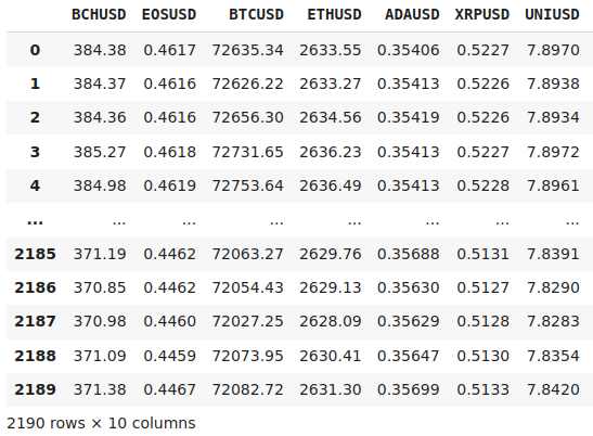
Fig 4: Visualizing some of the market data we have collected, recording 6 years of historic prices of a collection of cryptocurrencies

Exploratory Data Analysis

Trading cryptocurrencies can be challenging because the securities are very volatile. Fig 5, helps us visualize the performance of a basket of 10 cryptocurrencies over a 6-year period, from 2018 until 2024. The spread between the assets evolves and may not be intuitive for a human to calculate or use effectively.

data_plotting = data.iloc[:,:]/data.iloc[0,:]
sns.lineplot(data_plotting)

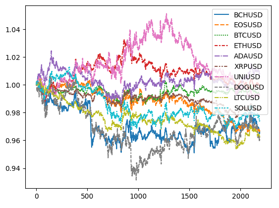
Fig 5: The performance of 10 different cryptocurrencies we could have invested in

The risk introduced into our portfolio by each cryptocurrency can be visualized as the rolling standard deviation of the returns of each Symbol. We can see from Fig 6 that periods of high volatility appear to cluster together. However, some markets exhibit more volatile behavior than other markets.

plt.plot(data_plotting.iloc[:,0].rolling(14).std())
plt.plot(data_plotting.iloc[:,1].rolling(14).std())
plt.plot(data_plotting.iloc[:,2].rolling(14).std())
plt.plot(data_plotting.iloc[:,3].rolling(14).std())
plt.plot(data_plotting.iloc[:,4].rolling(14).std())
plt.plot(data_plotting.iloc[:,5].rolling(14).std())
plt.plot(data_plotting.iloc[:,6].rolling(14).std())
plt.plot(data_plotting.iloc[:,7].rolling(14).std())
plt.plot(data_plotting.iloc[:,8].rolling(14).std())
plt.plot(data_plotting.iloc[:,9].rolling(14).std())
plt.legend(crypto)
plt.title("The Risk Associated With Each of our Cryptocurrencies")
plt.xlabel("Time")
plt.ylabel("Standard Deviation") 

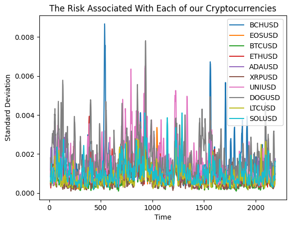
Fig 6: The standard deviation of each cryptocurrency in our portfolio

The PCA algorithm will help us intentionally minimize or maximize our exposure to the total variance of the portfolio being visualized in Fig 6. Trying to manually decide which assets will maximize our portfolio variance given 10 assets could prove impossible for a human being to do without help. 

Strong levels of correlation are somewhat expected when we analyze assets in the same asset class. Particularly interesting are the correlation levels between the:

1. EOSUSD & XRPUSD
   
2. DOGUSD & BCHUSD

These pairs are exhibiting almost perfect correlation levels over 6 years of Daily market quotes. This may be a relationship that our model can effectively use, and would be worth exploring under different circumstances.

#Correlation analysis
sns.heatmap(data.corr(),annot=True)

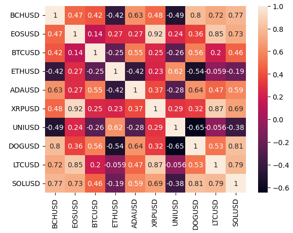
Fig 7: Visualizing the correlation levels in our portfolio of 10 cryptocurrencies

Calculate the change in price levels over 2 weeks.

#Calculate the change over 2 weeks
data = data.diff(14).dropna().reset_index(drop=True)

Now fit the scaler.

scaler = RobustScaler()
scaled_data = pd.DataFrame(scaler.fit_transform(data), columns=data.columns)

Fit the PCA object from scikit learn on our Daily market returns.

pca = PCA()
pca.fit(scaled_data)

Let us now analyze the first principal component. The sign of the coefficient instructs us if we should occupy long or short positions in each market. Positive coefficients tell us to go long, and negative coefficients instruct us to go short. Therefore, to maximize the variance of our portfolio, the PCA algorithm suggests going short across all the markets we have selected.

For traders who are looking to build scalping strategies, this first principal component is the way to go.

#High risk strategy
pca.components_[0]

array([-0.31760842, -0.32146743, -0.35867192, -0.35797826, -0.28276975, -0.36658864, -0.2954465 , -0.19875535, -0.32278201, -0.30604428])

Additionally, each component also provides us with optimal capital allocation ratios that will maximize or minimize the variance accordingly. However, to get this information, we must apply a few transformations to the component.

We will divide the component by its L1 Norm. The L1 Norm is the sum of absolute values in the component. By dividing each principal loading score by their total sum, we will know the optimal proportions we should allocate to each asset to maximize our portfolio variance.

After calculating the proportion of each cryptocurrency in the component, we can multiply the asset allocation ratio by the number of positions we want to open, to get an approximation of how many positions we should open in each market. We calculated the sum to prove that the total positions will add up to 100 if we multiply the asset allocation ratio by 100.

#High risk asset allocations can be estimated from the first principal component
high_risk_asset_allocation = pca.components_[0] / np.linalg.norm(pca.components_[0],1)
np.sum(high_risk_asset_allocation * 100)

-100

For example, if we wanted to open 10 positions following the high-risk strategy, our primary component suggests that we sell 1 position in BCHUSD (Bitcoin Cash). The decimal part of the coefficient can be interpreted as a position of a slightly smaller lot size. But this may prove significantly time-consuming to accurately consider in our portfolio. It may be simpler to rely on the whole number part of the allocation.

high_risk_asset_allocation * 10

array([-1.01533565, -1.02767219, -1.1466081 , -1.14439061, -0.90396285,-1.17191639, -0.94448806, -0.63538425, -1.03187466, -0.97836721])

Now let us move on to the medium risk principal components.

#Mid risk strategy
pca.components_[len(crypto)//2]

array([-0.00530455,  0.16374242,  0.03976866, -0.19508115,  0.75650629,0.08559565, -0.51882352, -0.15840483, -0.23524968,  0.06543203])

And finally, our low-risk principal components suggest an entirely different trading strategy all together.

#Low risk strategy
pca.components_[len(crypto)-1]

array([-0.03520096,  0.37157999, -0.41562007,  0.74700647, -0.06764155,-0.15451366, -0.28321595, -0.01342945, -0.09973515, -0.10555529])

Let us save these principal components to a text file, so we can use the findings in our MetaTrader 5 trading application.

np.savetxt("LOW RISK COMPONENTS.txt",pca.components_[len(crypto)-1])
np.savetxt("MID RISK COMPONENTS.txt",pca.components_[len(crypto)//2])
np.savetxt("HIGH RISK COMPONENTS.txt",pca.components_[0])

Implementing in MQL5

We are now ready to begin implementing Our MetaTrader 5 Trading Application

Our trading application will seek to follow the findings of our optimal asset allocations. We will open just 1 trade in each market according to the current risk setting the user has selected. The trading application will time its entries using the moving average and the Stochastic Oscillator.

If the principal component suggests that we enter long positions in the market, we will wait for price levels to rise above the moving average reading in that market and for the Stochastic Oscillator to be above 50. Once both our conditions are satisfied, we will take up our long position and accordingly set our take profit and stop loss levels using the ATR. Timing our market entries in this fashion should hopefully give us more stable and consistent entry signals over time.

To get started, we will first define the custom enumerator that gives our end user control over the risk parameters of our trading application.

//+------------------------------------------------------------------+
//|                               PCA For Portfolio Optimization.mq5 |
//|                                        Gamuchirai Zororo Ndawana |
//|                          https://www.mql5.com/en/gamuchiraindawa |
//+------------------------------------------------------------------+
#property copyright "Gamuchirai Zororo Ndawana"
#property link      "https://www.mql5.com/en/gamuchiraindawa"
#property version   "1.00"

//+------------------------------------------------------------------+
//| Custom enumerations                                              |
//+------------------------------------------------------------------+
enum risk_level
  {
   High=0,
   Mid=1,
   Low=2
  };

Load in the libraries we need.

//+------------------------------------------------------------------+
//| Libraries                                                        |
//+------------------------------------------------------------------+
#include  <Trade\Trade.mqh>
CTrade Trade;

Define constant values that will not change at any time.

//+------------------------------------------------------------------+
//| Constants values                                                 |
//+------------------------------------------------------------------+
const double high_risk_components[] = {#include "HIGH RISK COMPONENTS.txt"};
const double mid_risk_components[]  = {#include "MID RISK COMPONENTS.txt"};
const double low_risk_components[]  = {#include "LOW RISK COMPONENTS.txt"};
const string crypto[]               = {"BCHUSD","EOSUSD","BTCUSD","ETHUSD","ADAUSD","XRPUSD","UNIUSD","DOGUSD","LTCUSD","SOLUSD"};

Our global variables that we will use throughout our program.

//+------------------------------------------------------------------+
//| Global variables                                                 |
//+------------------------------------------------------------------+
double current_risk_settings[];
double vol,bid,ask;
int    atr_handler;
int    stoch_handler;
int    ma_handler;
double atr_reading[],ma_reading[],stoch_reading[];

We will allow the end user to dynamically control the risk settings of the trading account and the desired lot size.

//+------------------------------------------------------------------+
//| Inputs                                                           |
//+------------------------------------------------------------------+
input group "Risk Levels"
input risk_level user_risk = High; //Which risk level should we use?

input group "Money Management"
input int lot_multiple     = 1;    //How big should out lot size be?

When our trading application is loaded, we will first load our principal components according to the risk setting the user has selected. All of this will be taken handled for us by the "setup" function.

//+------------------------------------------------------------------+
//| Expert initialization function                                   |
//+------------------------------------------------------------------+
int OnInit()
  {
//--- Setup our market data
   setup();

//---
   return(INIT_SUCCEEDED);
  }

If we are no longer using the Expert Advisor, let us release the resources we are not using.

//+------------------------------------------------------------------+
//| Expert deinitialization function                                 |
//+------------------------------------------------------------------+
void OnDeinit(const int reason)
  {
//--- Release the indicators
   IndicatorRelease(atr_handler);
   IndicatorRelease(ma_handler);
   IndicatorRelease(stoch_handler);
  }

Finally, whenever we receive updated prices, let us maintain a portfolio of 1 position in each cryptocurrency market. The position we will occupy will be determined by the risk settings the user has selected. Depending on the risk setting, we may need to occupy a "buy" or "sell" position to control the variance in the portfolio.

//+------------------------------------------------------------------+
//| Expert tick function                                             |
//+------------------------------------------------------------------+
void OnTick()
  {
//--- Ensure we always have 10 positions
   if(PositionsTotal() < 10)
     {
      //--- Let's see which market we aren't in
      for(int i = 0; i < 10; i++)
        {
         //--- Check if we can now enter that market
         if(!PositionSelect(crypto[i]))
           {
            check_setup(i);
           }
        }
     }
  }

The setup function will determine which risk setting the end-user has selected and then load the corresponding principal component.

//+------------------------------------------------------------------+
//| Setup our market data                                            |
//+------------------------------------------------------------------+
void setup(void)
  {
//--- First let us define the current risk settings
   switch(user_risk)
     {
      //--- The user selected high risk
      case 0:
        {
         ArrayCopy(current_risk_settings,high_risk_components,0,0,WHOLE_ARRAY);
         Comment("EA in high risk mode");
         break;
        }
      //--- The user selected mid risk
      case 1:
        {
         ArrayCopy(current_risk_settings,mid_risk_components,0,0,WHOLE_ARRAY);
         Comment("EA in mid risk mode");
         break;
        }
      //--- The user selected low risk
      //--- Low risk is also the default setting for safety!
      default:
        {
         ArrayCopy(current_risk_settings,low_risk_components,0,0,WHOLE_ARRAY);
         Comment("EA in low risk mode");
         break;
        }
     }
  }

Since we are actively trading 10 different symbols, we need a function responsible for fetching market data related to each symbol. The "update" function defined below will handle this task for us. Whenever the function is called, it will load the current bid and ask price along with other technical indicator readings that are calculated from the specified market into memory. Once we have used the data and decided which action to take, the function will load the next Symbol's market data into memory.

//+------------------------------------------------------------------+
//| Update our system varaibles                                      |
//+------------------------------------------------------------------+
void update(string market)
  {
//--- Get current prices
   bid = SymbolInfoDouble(market,SYMBOL_BID);
   ask = SymbolInfoDouble(market,SYMBOL_ASK);
//--- Get current technical readings
   atr_handler   = iATR(market,PERIOD_CURRENT,14);
   stoch_handler = iStochastic(market,PERIOD_CURRENT,5,3,3,MODE_EMA,STO_CLOSECLOSE);
   ma_handler    = iMA(market,PERIOD_CURRENT,30,0,MODE_EMA,PRICE_CLOSE);
//--- Copy buffer
   CopyBuffer(atr_handler,0,0,1,atr_reading);
   CopyBuffer(ma_handler,0,0,1,ma_reading);
   CopyBuffer(stoch_handler,0,0,1,stoch_reading);
//---
  }

Finally, we need a function that will check if we can open a position aligned with the current risk settings the user has specified. Otherwise, if we cannot, we will give the end user a meaningful explanation why we cannot open a position in that market.

//+------------------------------------------------------------------+
//| Open a position if we can                                        |
//+------------------------------------------------------------------+
void check_setup(int idx)
  {
//--- The function takes the index of the symbol as its only parameter
//--- It will look up the principal component loading of the symbol to determine whether it should buy or sell
   update(crypto[idx]);
   vol = lot_multiple * SymbolInfoDouble(crypto[idx],SYMBOL_VOLUME_MIN);

   if(current_risk_settings[idx] > 0)
     {
      if((iClose(crypto[idx],PERIOD_D1,0) > ma_reading[0]) && (stoch_reading[0] > 50))
        {
         Comment("Analyzing: ",crypto[idx],"\nMA: ",ma_reading[0],"\nStoch: ",stoch_reading[0],"\nAction: Buy");
         Trade.Buy(vol,crypto[idx],ask,(ask - (atr_reading[0] * 3)),(ask + (atr_reading[0] * 3)),"PCA Risk Optimization");
         return;
        }
      else
        {
         Comment("Waiting for an oppurtunity to BUY: ",crypto[idx]);
        }
     }

   else
      if(current_risk_settings[idx] < 0)
        {

         if((iClose(crypto[idx],PERIOD_D1,0) < ma_reading[0]) && (stoch_reading[0] < 50))
           {
            Comment("Analyzing: ",crypto[idx],"\nClose: ","\nMA: ",ma_reading[0],"\nStoch: ",stoch_reading[0],"\nAction: Sell");
            Trade.Sell(vol,crypto[idx],bid,(bid + (atr_reading[0] * 3)),(bid - (atr_reading[0] * 3)),"PCA Risk Optimization");
            return;
           }

         else
           {
            Comment("Waiting for an oppurtunity to SELL: ",crypto[idx]);
            return;
           }
        }
   Comment("Analyzing: ",crypto[idx],"\nMA: ",ma_reading[0],"\nStoch: ",stoch_reading[0],"\nAction: None");
   return;
  };
//+------------------------------------------------------------------+

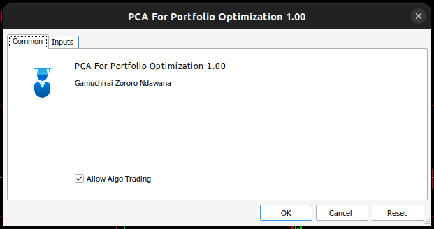
Fig 8: Viewing our expert advisor in MetaTrader 5

Fig 9: Adjusting the risk parameters of our trading application

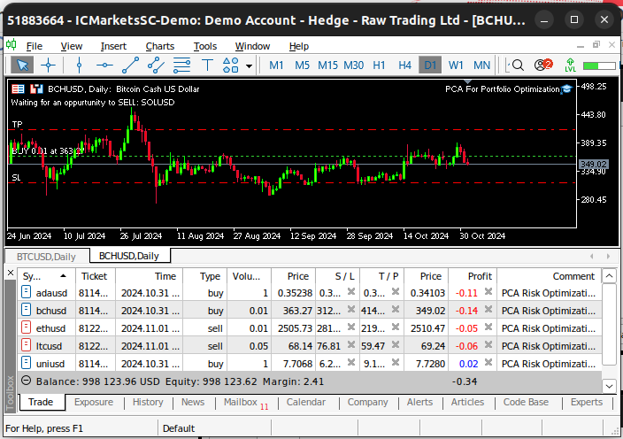
Fig 10: Our trading application being tested in real time on real market data

Conclusion

PCA is normally viewed as a somewhat complicated topic, due to the mathematical notation required to learn the concept. However, this article has hopefully shown you how to use PCA in an easy-to-use manner, that you can start applying today even if it is your first time learning about the topic.

Managing the risk in your portfolio allocation is not a simple task, mathematical tools and models are the best way of measuring and managing the risk you are exposed to in financial markets. Especially when the number of markets you wish to participate in grows large.

Whether we have 10 Symbols or 100 Symbols, PCA will always show us which combinations will maximize the risk in the portfolio and which combinations will minimize our portfolio risk.