MQL5 Wizard Techniques you should know (Part 11): Number Walls

Introduction

For a few time-series, it is possible to devise a formula for the next value in the sequences basing off of previous values that appeared within it. Number walls allow this to be accomplished by preliminarily generating a ‘wall of numbers’, in the form of a matrix via what is referred to as the cross-rule. In generating this matrix, the primary goal is to establish if the sequence in question is convergent and the number wall cross rule algorithm gladly answers this question, if after a few rows of application, the subsequent rows in the matrix are only zeroes.

In this published paper, that exhibits these concepts, the Laurent Power Series aka Formal Laurent Series (FLS) was used as a framework for representing these sequences with its arithmetic in polynomial format while using Cauchy products.

In general, LFSR sequences fulfill a recurrence relation such that the linear combination of consecutive terms is always zero as illustrated by the equation below:

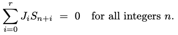
Where the sequence Sn is a linear recurring or linear feedback shift register (LFSR) and there exists a nonzero vector |Ji| (the relation) of length r + 1.

This implies a vector relation where the x coefficients (constants are coefficients of x to the power zero) constitute its elements. This vector by definition has a magnitude of at least 2.

To illustrate this, we can consider a couple of simple examples with the first being the sequence of cubed numbers. We all know cubed numbers enumerate from zero upwards with each value being a cube of its index position; and if we were to feed these into a number wall matrix, the initial representation would look as follows:

The zeroes and ones indicated as rows above the sequence are always implicit and they help in applying the cross rule so as to propagate all the missing values within the matrix. In applying the cross rule, for any 5 values in the matrix that are in a simple cross format, the product of the outer vertical values when added to the product of the outer horizontal values, should always be equivalent to the square of the center value.

If we apply this rule to the basic sequence of cubed numbers above we obtain the matrix represented below:

So to illustrate the cross rule, if we consider the number 216 in the sequence above 125 times 343, the numbers before and after it, when added to 7057 times 1, the numbers below and above it respectively, do give us the 216 to the power two.

The fact that we are able to so quickly obtain rows of zeroes signals that this sequence is indeed convergent, and a formula for its subsequent values can easily be derived.

But before we look at formulae let’s consider one more example, the Fibonacci series. If we are to apply this sequence in our matrix and apply the long cross rule as above, we obtain the rows of zeroes even quicker!

This certainly seems strange as one would expect the Fibonacci series to be more complex than cubed numbers and thus take longer to converge, but nope! it converges by the 2nd row.

To derive the formulation of a convergent series, such as the two examples considered above we would within the number wall matrix replace the sequence with a formulaic format that replaces any value in the sequence with the same value minus the value prior multiplied by x. This takes the following shape:

From here we simply apply our cross rule as we did with the sequences above and generate polynomial formatted values for the rows that follow. Interestingly enough if a sequence is convergent, even with the polynomial values we can still end up with rows of zeroes after a few propagations of the long cross rule. This is illustrated below for the Fibonacci sequence.

What then do we do with these polynomial values? Well it turns out if we equate the last equation to 0 and solve for the highest power of x, the x coefficients we are left with on the opposite side are multiples for previous values in the sequence that sum up to the next value.

So, with the last equation we got for the Fibonacci sequence if we solve for x^2 the highest power we are left with: 1 + x ;

Keep in mind that the 1 represents x^0 and is also in effect a coefficient to the sequence number before the sequence number whose coefficient is x. Put plainly what this says is in a Fibonacci series any number is the sum of two prior numbers in the sequence.

What does the polynomial equation for the cubed sequence look like? It takes more rows to converge as shown above and therefore it is more complex and rather than express the equation as a cube which is what you would expect.

How about non-convergent series what sort of matrices would one generate in these scenarios? To illustrate this perhaps we could jump right in by looking at the price sequence of a regular forex pair, take EURUSD. If we try to generate a number wall matrix, (without the formula) to test for convergence on a sequence of EURUSD daily close prices for the first 5 trading days of 2024 we would come up with a wall that resembles this for the first 5 rows.

As is self-evident we do not get convergence within the first rows in fact it is far from clear whether we ever do get strictly convergent, although the trend of the wall is towards zero so that should be comforting. This does dampen the applicability of number walls to our purposes and in fact this preliminary checking process is also typically compute intensive which is where the Toeplitz matrix comes into play.

If we create a matrix that has all rows related to each other in some way whereby we use a sliding repetition of the sequence row, if the sequence is convergent then the determinant of this matrix will be zero. This is a more compute efficient way for testing for convergence and more than that it ‘quantifies’ by how much we are likely to have a sequence converge based on the magnitude of the determinant.

So, we could propagate the cross rule on the formulaic matrix on any sequence and use the size of the determinant to ‘discount’ the forecast value of the formula. Alternatively, we can have an absolute threshold determinant value that if exceeded implies we ignore our formula result.

All these are possible work arounds non-convergent financial & other time series and they are certainly not perfect but let us examine what potential if any they have when implemented in MQL5.

MQL5 Implementation

To illustrate these ideas in MQL5 we’ll implement them in an instance of the Expert Trailing class that is paired with the inbuilt Awesome Oscillator Class to create a simple expert advisor. The instance of the trailing class will use the number wall to determine the size of the magnitude of the trailing stop loss and take profit level.

When implementing with MQL5, we will utilize the inbuilt data types of matrix and vector a lot given their extra functions and minimal code requirements. We can pre-screen a sequence for convergence by building a typical (non-formulaic) number wall and check if we arrive at a row of zeroes but given the nature and complexity of financial time series, it is a given the matrix will not converge and therefore we are better off computing the formula for the next value in the sequence as got from the bottom row of the last column after propagation.

To propagate the wall, we use vectors to store coefficients to x. Multiplying any two such vectors, in the process of solving for the unknown row would be equivalent to a cross correlation as the resulting vector values would be the x coefficients where a higher index placing indicates a higher exponent for x. This function is inbuilt however when it comes to division we need to resize the two quotient vectors to ensure they match up with any difference in size simply implying they do not match up in x exponents.

In determining by how much to adjust open position TP, and SL, our input sequence for our number wall will be indicator values of the moving average. Any indicator can be used although this or a Bollinger Bands or an Envelopes style indicator may be better suited in adjusting the trailing stop.

MQL5 vectors do easily copy and load indicator values once a handle is defined. If we look at the source below for a typical check trailing stop code (usable for both long and short)

//+------------------------------------------------------------------+
//| Checking trailing stop and/or profit for long position.          |
//+------------------------------------------------------------------+
bool CTrailingLFSR::CheckTrailingStopLong(CPositionInfo *position, double &sl, double &tp)
{
//--- check

...

//---
   vector _t, _p;
   _p.Init(2);
   _t.CopyIndicatorBuffer(m_ma.Handle(), 0, 0, 2);
   double _s = 0.0;
   for(int i = 1; i >= 0; i--)
   {  _s = 0.0;
      _p[i] = GetOutput(i, _s);
   }
   double _o = SetOutput(_t, _p);
//---
  
...

}

We can see our decision making is evolving around two functions, the get output and set output. The get output is the primary as it builds the number wall and comes up with polynomial coefficients to an equation that solves for the next value in the sequence. The get output listing as indicated below:

//+------------------------------------------------------------------+
//| LFSR Output.                                                     |
//+------------------------------------------------------------------+
double CTrailingLFSR::GetOutput(int Index, double &Solution)
{  double _output = 0.0;
   vector _v;
   _v.CopyIndicatorBuffer(m_ma.Handle(), 0, Index, m_length);
   Solution = Solvability(_v);
   _v.Resize(m_length + 1);
   for(int i = 2; i < 2 + m_length; i++)
   {  for(int ii = 2; ii < 2 + m_length; ii++)
      {  if(i == 2)
         {  vector _vi;
            _vi.Init(1);
            _vi[0] = _v[m_length - ii + 1];
            m_numberwall.row[i].column[ii] = _vi;
         }
         else if(i == 3)
         {  vector _vi;
            _vi.Init(2);
            _vi[0] = m_numberwall.row[i - 1].column[ii][0];
            _vi[1] = -1.0 * m_numberwall.row[i - 1].column[ii - 1][0];
            m_numberwall.row[i].column[ii] = _vi;
         }
         else if(ii < m_length + 1)
         {  m_numberwall.row[i].column[ii] = Get(m_numberwall.row[i - 2].column[ii], m_numberwall.row[i - 1].column[ii - 1], m_numberwall.row[i - 1].column[ii + 1], m_numberwall.row[i - 1].column[ii]);
         }
      }
   }
   vector _u = Set();
   vector _x;
   _x.CopyIndicatorBuffer(m_ma.Handle(), 0, Index, m_length);
   _u.Resize(fmax(_u.Size(),_x.Size()));
   _x.Resize(fmax(_u.Size(),_x.Size()));
   vector _y = _u * _x;
   _output = _y.Sum();
   return(_output);
}

Our shared listing above is basically 2 part. Building the wall to get the equation coefficients, and using the equation with the current sequence readings to project. In the first part the get function is key multiplying generated equations and solving for the equation for the next row. The listing is given below:

//+------------------------------------------------------------------+
//| Get known Value                                                  |
//+------------------------------------------------------------------+
vector CTrailingLFSR::Get(vector &Top, vector &Left, vector &Right, vector &Center)
{  vector _cc, _lr, _cc_lr, _i_top;
   _cc = Center.Correlate(Center, VECTOR_CONVOLVE_FULL);
   _lr = Left.Correlate(Right, VECTOR_CONVOLVE_FULL);
   ulong _size = fmax(_cc.Size(), _lr.Size());
   _cc_lr.Init(_size);
   _cc.Resize(_size);
   _lr.Resize(_size);
   _cc_lr = _cc - _lr;
   _i_top = 1.0 / Top;
   vector _bottom = _cc_lr.Correlate(_i_top, VECTOR_CONVOLVE_FULL);
   return(_bottom);
}

Likewise, the set function uses the bottom vector, that has the last propagated coefficients to solve the next sequence value and its listing is shared below:

//+------------------------------------------------------------------+
//| Set Unknown Value                                                |
//+------------------------------------------------------------------+
vector CTrailingLFSR::Set()
{  vector _formula = m_numberwall.row[m_length + 1].column[m_length + 1];
   vector _right;
   _right.Copy(_formula);
   _right.Resize(ulong(fmax(_formula.Size() - 1, 1.0)));
   double _solver = -1.0 * _formula[int(_formula.Size() - 1)];
   if(_solver != 0.0)
   {  _right /= _solver;
   }
   return(_right);
}

Now within a check trailing function we call the get output function twice because we need to get not just the current forecast but also the prior to aid in normalizing our outputs this is because since most sequences and especially financial time series do not converge, as mentioned in the intro, the raw output forecast is bound to be a very alien figure to the input sequence values. Getting very large double values several magnitudes of the typical sequence values or even a negative value when obviously only positive values are expected, is not uncommon.

So, in normalizing we use the very brief and simple set output function which is shared below:

//+------------------------------------------------------------------+
//| Normalising Output to match Indicator Value                      |
//+------------------------------------------------------------------+
double CTrailingLFSR::SetOutput(vector &True, vector &Predicted)
{  return(True[1] - ((True[0] - True[1]) * ((Predicted[0] - Predicted[1]) / fmax(m_symbol.Point(), fabs(Predicted[0]) + fabs(Predicted[1])))));
}

All we are doing is simply normalizing the projected value to have its magnitude within the range of the sequence values and we achieve this by utilizing sequence changes for both the predicted and the true.

Also, in the typical check trailing stop we do measure for solvability within the get output function at its onset. This metric is used as a threshold filter to determine whether we should ignore the forecast with the thesis being larger determinant values (what we are referring to as solvability) indicate higher inability to converge. Suffice it to say even a matrix with a small determinant does not converge however we assume that it is more likely to converge, when provided with more rows to build the number wall, than a matrix with a higher determinant.

So, putting this all together gives us the instance of the trailing class attached at the end of the article and although preliminary testing does indicate it is compute-intense & it does, in my opinion, present an idea that could be honed and even paired with different strategies to develop a more robust trade system.

The attached code to the trailing class in MQL5 can easily be assembled with a wizard to create a variety of expert advisors depending on the choice of signal class and money management. As always help is here as a guide on how to go about this.

Additional notes

The number walls considered this far in the shared code and above illustrations used whole security prices which did not include any zeroes. If we for instance want to forecast changes in the security price and not just the raw price we would ideally have an input series of price changes. Once we begin dealing with changes as opposed to the absolute price we not only run into negative values, but we can also, and are bound to have quite often, a few zeroes.

Initially zeroes may seem harmless but when we are building number walls they do present challenges in determining the values on the next row. Consider the following example:

With our basic cross rule in solving for the unknown value we run into a problem since one known value is zero and therefore when multiplied with our unknown leaves us empty handed. To circumnavigate this, the log cross rule comes in handy. And here is its representation if we expand the image above:

We can with some confidence work around the zero above our current row by exercising the formula below:

I mention with ‘some confidence’ because number walls have a very unique property when it comes to including zeroes. It turns out in any number if there are zeroes then they occur singularly or in a square form meaning they can be 1 x 1 (singular) or 2 x 2, or 3 x 3, and so on. This basically means if we come across a zero between two numbers on any row, then the number below it is not a zero. Anyone can see though that as we apply the long cross rule we have an extra unknown in the form of the lowest outer value in the wall. This is not a problem though as it is multiplied by our known zero which allows us to solve the equation without having to input its value.

The problem addressed by the long cross rule applies strictly to converging number walls and as we’ve seen with our illustrations above this is rarely the case with financial time series. So, should this be considered? This honestly should be determined on a sequence by sequence basis depending on the time series a trade system is focused on. Some could choose to apply it even on financial series if the ‘solvability’ or Toeplitz matrix determinant meets a necessary threshold, others could terminate building the wall and work with the vector coefficients they have at that point (when they run into zeroes) in building the forecast polynomial equation. There are these and perhaps a few other options and the choice will be trader specific.

The long cross rule is resourceful if one encounters just the one zero when propagating a number wall however if the zeroes are in a larger square (since zeroes always take up the n x n format in a wall) Then it would not be of much use and in these instances, what is often considered is the horse shoe rule. With this rule typically once you have a large square of zeroes, the bordering sequences to this square have their values scaled by a specific factor.

These four factors, one to each side of a square, share a unique property that can be summed up by the formula below:

So, when a large tranche of zeroes is encountered the top and side numbers that border these zeroes would already be known and since we know the width of the zeroes squares we in essence know its height meaning we know where to evaluate the unknown border values. From the above equation the immediate border values below can be got from working out the bottom scale factor and computing its numbers, typically from left to right.

However, progressing from this point with the ordinary cross rule would still be difficult as the zeroes in the square make its application difficult in determining the row below the just solved border row. Resolving this represents the ‘second part’ of the horse shoe rule and it relies of the following somewhat lengthy formula:

The already referenced paper above on this subject, in addition to highlighting many of the points shared here, also talks a bit about the pagoda conjecture. In its simplest form this is the summation of a group of sets of numbers with each contained set being of equal size such that if each of the included sets is construed as a polygon with each vertex representing one of the numbers in its set then these polygons can be glued together to form a larger complex lattice with the condition that at any linked vertex all polygon vertices have the same number. This of course happens with the condition that each vertex number on any one polygon is unique within that set.

This has firstly interesting picturesque consequences for 3-number sets that form a pagoda as it turns out when each set’s numbers are outlaid in a sequence very interesting repetitive patterns can be observed in the propagated number wall from it and the paper shares some of these images.

For trading purposes though this ‘novel’ approach at classification does present yet another way of looking at financial time series which to be honest should require an independent article but suffice it to say we could generalize a few ways we could apply pagoda sequences to our uses.

Off the cuff if we are going to apply this it could be prudent to stick to triangular pagodas as opposed to higher dimension forms as these tend to raise more possibilities and therefore complexity on how they can be joined. If we could accept this then our task would be firstly to normalize our financial series to accommodate the repetition of values which is a requirement when defining the pagodas as highlighted already and the degree to which this normalization is done is something that would need to be examined carefully since different iterations are bound to yield different results.

Secondly, once we are comfortable with a certain normalization threshold, we would need to set the number of triangles in our pagoda, i.e. the group size. Keep in mind that as the group size increases the need to all triangle to be directly linked diminishes so in a 3-triangle pagoda, all triangles are linked but as this number increases then for any triangle the most linkages it can have is 3 meaning say a 6-triangle pagoda only the bottom central triangle has links on all its vertices with all the others having links on only two vertices.

This increasing complexity on the joining of the triangles, with increasing group size, could suggest that determining the optimal group size should be done in tandem with setting the normalization threshold since the later gives us our repeated data that is key in establishing the links across the triangles.

Conclusion

To conclude we have looked at number walls, a grid of numbers generated from a sequence time series under examination, and seen how it could be used in forecasting by properly setting open position TP & SL in the shared code example. In addition, we have looked at the related concept of pagoda conjectures which were the highlight of a paper on number walls, and put forward some ideas how they could be another avenue in classifying financial time series.

Epilogue

Comparative tests of wizard assembled expert advisers are shown below. They both use the awesome oscillator signal and in principal have simillar inputs as indicated here:

The difference betwen them is one expert uses the parabolic sar to trail and close open positions while the other uses the number wall algorithm introduced in this article. However their reports when tested on EURUSD over the past year on the hourly time frame, despite the same signal, do differ. First below is the parabolic sar trailing stop expert.

And the number wall report is also indicated below:

The overall difference in result is not significant, but it could be critical if tested and tried not only over longer periods, but also in different expert classes like money management or even signal generation.