Forecasting Realized Volatility with Option-Implied Variance for Multiple Instruments in MQL5
 86
 0

Introduction
Most volatility models in a trading terminal use only the price history of the symbol on the chart. The options market adds a second view every day: the price it charges for protection over the next month. This article tests whether that view improves forecasts of realized volatility. It does: across four markets with Cboe volatility indices and ten US equities with option chains, a HAR model with an implied term beat plain HAR out of sample. In the markets and stocks tested, the gain was largest where price history alone forecast worst.
The design follows one line. Python supplies only what the terminal cannot measure, a daily history of option-implied variance. MQL5 fits the model on the broker's own bars and shows the scale of the expected move on the chart. None of it trades.
The attachments include a feed script, a forecasting class for MQL5, a check script that validates the class against independent C++ and Python implementations, a background service with a chart panel, the research scripts behind the main tests, and a file of supplementary results.
Model and realized-variance measurement
Realized volatility is what the instrument actually did, measured from prices after the fact. It is the quantity being forecast. Implied volatility is what the options market charges for the next thirty days, and a Cboe volatility index computes it from a strip of option prices. [7] It is a risk-neutral price: it includes the compensation sellers demand for providing protection, the variance risk premium, so it usually sits above the volatility later realized. [6] The model therefore does not take implied volatility as a ready-made forecast. It uses it as one predictor among four and lets the regression decide its weight.
Each implied series is built from options on a fund or index, not on a symbol a broker quotes:
| Market | Implied series | Built from options on | Feed file | Typical broker symbol |
|---|---|---|---|---|
| Gold | GVZ | GLD, a gold ETF | vol_gld.json | XAUUSD |
| S&P 500 | VIX | SPX, the S&P 500 index (diagnostics on SPY) | vol_spy.json | US500 |
| Crude oil | OVX | USO, an oil futures fund | vol_uso.json | USOIL |
| Nasdaq-100 | VXN | NDX, the Nasdaq-100 index (diagnostics on QQQ) | vol_qqq.json | US100 |
These pairings are proxies. How the model deals with that is the subject of the next section.
Corsi's heterogeneous autoregressive model, HAR, forecasts realized variance from its own averages over the last one, five, and twenty-two sessions. [1] Adding the implied term gives the model tested here, with h the horizon in sessions:
log RV(t+1..t+h) = b0 + b1 * log RV1(t) + b5 * log RV5(t) + b22 * log RV22(t) + bIV * log IV(t)
RV1, RV5, and RV22 are the annualized trailing averages ending at session t. IV is the implied variance already published when session t closed. Logarithms keep a few crisis days from dominating the fit. Implied volatility is known to carry information about future realized volatility, [4] and it has been added to HAR regressions before. [5] What is new here is running the model inside the terminal on the broker's bars. The model works in variance, while the panel reports volatility, its square root. The default horizon is five sessions.
Measuring the realized side took two failed attempts. Squared close-to-close returns were too noisy. Garman-Klass, built from the open, high, low, and close, is far quieter, [2] but it sees only the hours the market is open. On SPY, 43.2 percent of daily variance arrives between one close and the next open, so Garman-Klass alone understated the total by more than forty percent. The estimator used here adds the overnight gap back:
daily variance = log(open / previous close)^2 + 0.5 * log(high / low)^2 - (2 * log(2) - 1) * log(close / open)^2
In the engine, it is one short function:
double CVolatilityForecast::DailyVariance(const double prev_close, const MqlRates &r)
  {
   if(prev_close <= 0.0 || r.open <= 0.0 || r.high <= 0.0 ||
      r.low <= 0.0 || r.close <= 0.0)
      return(-1.0);

   double overnight = MathLog(r.open / prev_close);
   double ln_hl     = MathLog(r.high / r.low);
   double ln_co     = MathLog(r.close / r.open);
   double garman    = 0.5 * ln_hl * ln_hl
                      - (2.0 * MathLog(2.0) - 1.0) * ln_co * ln_co;
   return(overnight * overnight + garman);
  }
On a symbol that trades around the clock, the open sits on the previous close, and the first term falls to zero by itself, so the same expression serves every venue. A day whose total comes out negative can only come from a damaged bar and is treated as missing.
Why the model is fitted on broker bars
Funds and around-the-clock contracts split the same daily variance differently. The table measures the overnight share with the same estimator from 2019 onward. Futures stand in for broker contracts because their history is free, and the last two rows come from the author's broker through the MQL5 engine, over up to 3,000 daily bars of each symbol:
| Venue | Instrument | Session length | Overnight share of daily variance (%) |
|---|---|---|---|
| Fund | GLD | 6.5 hours | 59.1 |
| Fund | SPY | 6.5 hours | 43.2 |
| Fund | USO | 6.5 hours | 52.8 |
| Fund | QQQ | 6.5 hours | 41.0 |
| Futures | GC gold | about 23 hours | 13.6 |
| Futures | ES S&P 500 | about 23 hours | 9.5 |
| Futures | CL crude oil | about 23 hours | 15.8 |
| Futures | NQ Nasdaq-100 | about 23 hours | 8.0 |
| Broker | XAUUSD | about 24 hours | 2.4 |
| Broker | US500.cash | about 24 hours | 5.4 |
Every fund is above 41 percent, and every future is below 16 percent, while total volatility agrees: SPY realized 19.5 percent a year against 19.2 for ES. This does not prove that coefficients fitted on fund bars would fail on a broker symbol, but it is a strong reason not to assume they transfer. The design therefore keeps the two sides apart:
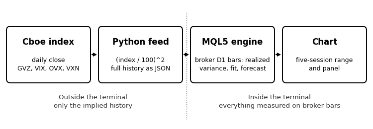
Python publishes the implied history and nothing else. MQL5 measures realized variance, fits the coefficients, and forecasts on the terminal's own bars.
The implied series crosses from the option market only as information. The attached overnight_share.py reproduces the table above, and the broker results in the next section test the local fit out of sample.
Out-of-sample results
Every forecast below is made out of sample by a model refitted on an expanding window. A training row enters only after its forward window has closed. Out-of-sample R-squared compares each forecast with the expanding historical mean. The Clark-West test, built for nested models, [3] gives one-sided p-values for whether the implied term helps. Forecast windows longer than one session overlap, so the tests use Newey-West errors with 2(h - 1) lags. The main horizon is five sessions. Results at one, five, and twenty-two sessions, with 4(h - 1) lags and on non-overlapping windows, are in supplementary_results.txt.
On SPY, with implied variance rebuilt from option chains, adding the implied term improved five-session out-of-sample R-squared by 5.6 percentage points over the development period, May 2019 to June 2025 (Clark-West t 4.91), and by 7.2 points on a holdout from July 1, 2025, to September 4, 2026, which was opened once after development ended (t 3.68). The improvement remained significant with twice the Newey-West lags and on non-overlapping windows. A favorable holdout period could produce the same pattern, so this is consistent with a result that is not overfitted, not proof of it. The twenty-two-session horizon was declared underpowered in advance, because the holdout holds only thirteen non-overlapping twenty-two-session periods, and it is not used for any conclusion.
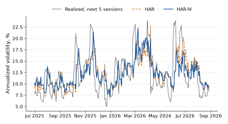
Five-session forecasts on the SPY holdout, July 1, 2025, to September 4, 2026, from models refitted every session. HAR uses price history alone; HAR-IV adds the implied term. The plotted quantity is volatility, not price.
The two forecasts differ most around spikes. HAR responds only once a spike enters the trailing averages, while the implied term carries what the options market was already pricing.
The option database has no gold chains, so the second test used Cboe indices: four funds paired with their indices from January 2015 to September 4, 2026, scoring the last sixty percent of each sample, 1,746 five-session forecasts per market. All twelve comparisons across the three horizons are positive, with p-values below 0.0001. At five sessions:
| Market | Fund / index | HAR R-squared (%) | HAR-IV R-squared (%) | Gain (points) | Clark-West t |
|---|---|---|---|---|---|
| Gold | GLD / GVZ | 47.2 | 54.9 | +7.8 | 6.15 |
| Crude oil | USO / OVX | 51.4 | 57.4 | +5.9 | 7.14 |
| S&P 500 | SPY / VIX | 58.7 | 63.7 | +5.1 | 6.67 |
| Nasdaq-100 | QQQ / VXN | 60.4 | 64.8 | +4.5 | 6.19 |
The VIX row is a consistency check, not a control: the chain-built SPY series gave +5.6 points against +5.1 here. Agreement between two sources does not prove that either is free of errors. har_iv_research.py reproduces this table from free data.
The ten-equity test used weekly option chains. The data and filters are summarized below; the full specification is in section S4 of supplementary_results.txt, and har_iv_chains.py reproduces the test from the same source, with the implied variance built in its functions variance_for and svix_for_day:
| Item | Setting |
|---|---|
| Source | Dolt database post-no-preference/options, table option_chain (https://www.dolthub.com/repositories/post-no-preference/options), DoltHub SQL API, branch master, downloaded September 6 to 8, 2026 |
| Sampling | Wednesdays, January 1, 2020, to September 4, 2026 |
| Quote filter | bid > 0, mid >= 0.05, and (ask - bid) / mid <= 0.25 |
| Implied variance | Out-of-the-money Black-76 prices around a put-call parity forward, integrated as 2 / (t * F^2) * integral of price over strike, interpolated to 30 days |
| Exclusion rule | Fewer than 120 Wednesdays with a usable implied variance, applied before any forecast was fitted |
| Candidates | The 31 large US option markets the database carried on September 4, 2026: META, MSFT, XLK, CAT, XLV, SPY, AAPL, TSLA, XLE, JPM, GOOGL, NVDA, IBM, MCD, AMZN, CSCO, INTC, XLF, DIA, GE, WMT, DIS, BA, KO, JNJ, VZ, XOM, BAC, PFE, T, NKE |
| Fixed in advance | SPY, DIA, XLF, XLE, XLK, AAPL, MSFT, JPM, XOM, KO |
| Added later | NVDA, GOOGL, AMZN, CAT |
| Passed | SPY, DIA, AAPL, MSFT, JPM, XOM, NVDA, GOOGL, AMZN, CAT |
| Excluded | XLF, XLE, XLK, KO (median quoted spreads 20 to 25 percent of the option price) |
All ten symbols that passed improved at both one and five sessions, with Clark-West p-values below 0.01. Weekly sampling means the five-session windows never overlap. The six that came from the list fixed in advance are all positive. Ten out of ten is descriptive, not a test, because the names share one market factor, one data source, and one period.
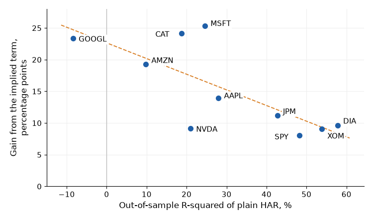
Each point is one symbol at the five-session horizon. The horizontal axis shows how well plain HAR forecasts on its own; the vertical axis shows how much the implied term adds. The dashed line is a least-squares fit across the ten points.
Across the ten symbols, the correlation between plain HAR strength and the gain is -0.74 at five sessions (two-sided p = 0.014, Student's t-test with 8 degrees of freedom) and -0.59 at one session (p = 0.07, not significant). On GOOGL, plain HAR scores -8.4 percent, worse than the historical mean, and HAR-IV reaches 15.0 percent. Scheduled earnings, which option prices can include and trailing prices cannot, are one plausible explanation for single stocks, not a proven one. Gold shows the same pattern in the four-market table, and the reason there is not established.
The engine repeats the test on broker bars. These rows are a demonstration using the author's data, not a reproducible experiment. They come from one retail broker's MetaTrader 5 server, whose clock was UTC+3 on the test date, so its daily bar closed at 17:00 New York time and needed no implied lag. The symbols are that broker's XAUUSD and US500.cash, with up to 3,000 daily bars ending September 25, 2026, the default of the check script, matched to the feeds from January 2015. The bars themselves are not published. The last 60 percent of rows were scored:
| Chart and feed | Observations | Forecasts scored | HAR R-squared (%) | HAR-IV R-squared (%) | Gain (points) | Clark-West t |
|---|---|---|---|---|---|---|
| XAUUSD with the GLD feed | 2,895 | 1,737 | 52.0 | 61.6 | +9.7 | 6.62 |
| US500.cash with the SPY feed | 2,172 | 1,304 | 50.9 | 58.4 | +7.5 | 8.72 |
Two symbols on one broker are not a general result. They show only that the gain is not confined to the fund data where it was first measured.
A better forecast did not become a trading edge. Six rules used the SPY forecast to decide when to sell volatility, and a control sold whenever implied variance was in its top third, using no model. The payoff was a proxy: implied minus realized variance over the next 22 sessions, divided by implied variance, roughly what a variance swap earns, with no costs modeled. The 581 forecasts are dated January 3, 2022, to June 30, 2025. "Raw" uses the exponential of the log forecast, and "smeared" applies Duan's correction, because the exponential of a forecast of a log understates the level. The full specification is in section S6 of the supplementary file.
Rule Uses the model Days active Mean payoff = break-even cost (%) Sharpe ratio Worst period (%) A. Short every day No 581 6.1 0.35 -633.6 D. Short when implied is in its top third (control) No 194 8.7 0.63 -386.9 B. Short when implied exceeds the forecast, raw Yes 551 4.8 0.29 -633.6 C. Short when implied over forecast is in its top third, raw Yes 194 9.1 0.49 -314.4 E. Short when implied exceeds the forecast, long otherwise, raw Yes 581 3.0 0.22 -633.6 B. As B, smeared forecast Yes 54 11.7 0.40 -260.7 C. As C, smeared forecast Yes 194 5.3 0.23 -361.3 E. As E, smeared forecast Yes 581 -3.9 -0.23 -260.7
| Rule | Uses the model | Days active | Mean payoff = break-even cost (%) | Sharpe ratio | Worst period (%) |
|---|---|---|---|---|---|
| A. Short every day | No | 581 | 6.1 | 0.35 | -633.6 |
| D. Short when implied is in its top third (control) | No | 194 | 8.7 | 0.63 | -386.9 |
| B. Short when implied exceeds the forecast, raw | Yes | 551 | 4.8 | 0.29 | -633.6 |
| C. Short when implied over forecast is in its top third, raw | Yes | 194 | 9.1 | 0.49 | -314.4 |
| E. Short when implied exceeds the forecast, long otherwise, raw | Yes | 581 | 3.0 | 0.22 | -633.6 |
| B. As B, smeared forecast | Yes | 54 | 11.7 | 0.40 | -260.7 |
| C. As C, smeared forecast | Yes | 194 | 5.3 | 0.23 | -361.3 |
| E. As E, smeared forecast | Yes | 581 | -3.9 | -0.23 | -260.7 |
No model rule beat the control's Sharpe ratio of 0.63, although two earned a higher mean payoff. This concerns six rules under one cost-free payoff. It does not show that no edge can be built on the forecast.
Implementation in Python and MQL5
MetaTrader cannot read Cboe indices, so volatility_forecast_feed.py downloads the matching index for GLD, SPY, USO, or QQQ, converts each daily close to annualized variance as (index / 100)^2, and publishes one flat JSON file with every session since January 2015, about 2,950 of them. The history travels in two comma-separated fields, dates and values, next to fields such as asof, index, and local_symbol_hint, so a small MQL5 reader can split it directly. That reader handles only this flat format: no escaped quotes, nested objects, or arrays. The file also carries reference figures measured on the fund's own bars, such as ref_premium_win_full, the share of dates on which implied variance exceeded the realized variance of sessions t+1 to t+21. Dates without a complete forward window are dropped. These figures describe the fund and are not used by the terminal. Their current values are in section S7 of the supplementary file. A failed download leaves the previous file untouched. A GitHub Actions workflow, saved as .github/workflows/update-volatility-feeds.yml, rebuilds the four feeds at 21:30 and 23:30 UTC every weekday and can be started by hand from the Actions tab with "Run workflow." The workflow is attached as update-volatility-feeds.txt, and the published feeds are in the repository https://github.com/GeneTheStoic/volatility-forecast-feed.
The feed needs the whole history, not just today's value. An early MQL5 draft used today's implied value on every historical row, which made the implied column constant, identical in shape to the intercept, and the regression singular.
A daily bar dated D closes at the server's midnight, and the index for D is final at 16:15 New York time. If the bar closes first, pairing it with that day's quote would use information from the future, so each bar takes the previous bar's quote instead:
#define HARIV_CBOE_CLOSE 58500    // 16:15 New York, in seconds after midnight

int CVolatilityForecast::SuggestedLag(void)
  {
   return(BarCloseNewYork() * 3600.0 < HARIV_CBOE_CLOSE ? 1 : 0);
  }
BarCloseNewYork converts the server's midnight to New York time with the US daylight-saving rule, and the calendar helpers are in the attached file. A server whose clock does not follow US daylight saving can close before the index in one season and after it in the other and should set the lag by hand. Each bar is then matched to the quote carrying its own server date, shifted by the lag. A bar without a quote is left out of the fit rather than given an older value. Only the forecast origin may borrow the last published quote, up to four days old, when a US holiday leaves the newest bar without one.
CVolatilityForecast in VolatilityForecastEngine.mqh holds all of the mathematics, and both programs include it. In use, it needs only a few calls:
CVolatilityForecast engine;
engine.Init(_Symbol, PERIOD_D1, 5, 3000);   // symbol, timeframe, horizon, bars
engine.SetImplied(times, values, count);    // the feed's dates and variances
engine.SetImpliedLag(CVolatilityForecast::SuggestedLag());
if(engine.Calculate())
   PrintFormat("Forecast %.2f%%, implied %.2f%%, %d observations",
               engine.ForecastVol(), engine.ImpliedVol(), engine.Rows());
else
   Print(engine.StateText());
Calculate fits by Householder QR, which works on the design matrix directly, because forming the normal equations would square the condition number of correlated HAR terms. It then forecasts from the newest complete bar. OutOfSample then repeats the research design on the same bars. Rows are kept in bar order, so the training set for row k is the prefix of rows whose forward windows had closed by row k's date, and each scored row adds one Clark-West term:
   for(int k = first; k < m_nrows; k++)
     {
      int n = 0;
      while(n < k && m_row_at[n] + h <= m_row_at[k])
         n++;
      if(n < HARIV_MIN_ROWS)
         continue;
      double s1 = 0.0, s2 = 0.0;
      if(!LeastSquares(n, HARIV_NPARAM - 1, bh, s1) ||
         !LeastSquares(n, HARIV_NPARAM, bf, s2))
         continue;
      //--- ...the HAR and HAR-IV forecasts of row k (ph, pf) and its outcome a
      f[scored] = (a - ph) * (a - ph) - (a - pf) * (a - pf) + (ph - pf) * (ph - pf);
      scored++;
     }
The full test, with the Newey-West step that turns these terms into a t statistic, is in the attached file.
A hand-written solver can fail without saying so, so the same model was solved three ways on one deterministic synthetic series: in MQL5 by Householder QR, in a C++ reference by Gaussian elimination, and in Python with NumPy. The three agree to ten decimals:
| Implementation | Solver | Rows | b0 | b1 | b5 | b22 | bIV |
|---|---|---|---|---|---|---|---|
| MQL5 engine, self-test | Householder QR | 573 | 0.7203612679 | 0.0158634226 | -0.0904041218 | 0.1115491403 | 0.9119636554 |
| C++ reference | Gaussian elimination | 573 | 0.7203612679 | 0.0158634226 | -0.0904041218 | 0.1115491403 | 0.9119636554 |
| Python, har_iv_check.py | NumPy least squares | 573 | 0.7203612679 | 0.0158634226 | -0.0904041218 | 0.1115491403 | 0.9119636554 |
VolatilityForecastCheck.mq5 runs this self-test by default; har_iv_check.py is the Python side. With InpSelfTest set to false, the script reads a feed file from MQL5\Files and prints the server's daily close in New York time, the forecast, and the out-of-sample test on the chart's symbol.
Installation and chart panel
Unpack MQL5.zip into the terminal data folder. The engine goes to MQL5\Include\VolatilityForecast, the script to MQL5\Scripts\VolatilityForecast, and the service to MQL5\Services\VolatilityForecast. Compile both programs with F7. In "Tools," "Options," "Expert Advisors," enable "Allow WebRequest for listed URL" and add https://raw.githubusercontent.com. Open the chart of the symbol to monitor, right-click VolatilityForecastService under Services in the Navigator, and choose "Add Service." Set FeedURL to https://raw.githubusercontent.com/GeneTheStoic/volatility-forecast-feed/main/ followed by the feed file from the market table in the first section, and LocalSymbol to the exact name in Market Watch, including any suffix such as .cash. Add the service once per pair to watch several markets. A mismatched pair is the one error the program cannot detect.
Every hour, the service reads the feed, refits on the broker's daily bars, and redraws the chart. ImpliedLag is -1 by default, which picks the lag from the server clock at every reading. The forecast becomes a price distance once, in the panel:
band = bid * forecast volatility * sqrt(horizon / 252)
The volatility enters as an annualized decimal, and dashed lines are drawn one band above and below the bid. The band is a scale of the typical move: it is not a probability interval, it ignores direction and skew, and its coverage has not been calibrated. The panel adds two words. Movement compares the forecast with last week's realized variance and reads BUILDING or EASING only when the difference exceeds the fit's own typical error, STEADY otherwise. Option price ranks today's ratio of implied to forecast volatility within the symbol's fitted history: the lowest third reads CHEAP, the highest third EXPENSIVE, and the rest FAIR. Both are conventions, not statistical tests, and the R-squared on the panel is in-sample.
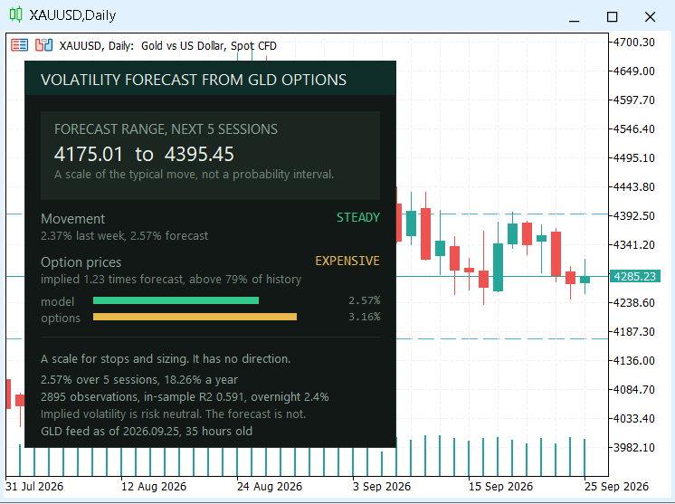
The service on the broker's XAUUSD chart with the GLD feed, after the close of September 25, 2026.
The two panels from that day read:
| Chart and feed | Forecast, a year (%) | Forecast, 5 sessions (%) | Options, 5 sessions (%) | Implied over forecast | Rank in own history (%) | Observations | In-sample R-squared | Overnight share (%) |
|---|---|---|---|---|---|---|---|---|
| XAUUSD with the GLD feed | 18.26 | 2.57 | 3.16 | 1.23 | 79 | 2,895 | 0.591 | 2.4 |
| US500.cash with the SPY feed | 9.84 | 1.39 | 2.09 | 1.51 | 74 | 2,172 | 0.615 | 5.4 |
These are one day's readings, not properties of either market. Both read EXPENSIVE and STEADY. Each panel measures the overnight share on its own broker history.
Interpretation and limitations
The most direct use is stop distance. ATR and trailing volatility look only backward, while the band includes what options are pricing about the days ahead, so a stop inside it should be a deliberate choice. The same number can size a position so that a move of the forecast size costs a fixed amount. In both uses, it is a scale, not a loss probability.
Limits not covered above:
- The option-chain source can carry stale quotes and reconstructed mid prices, and survivorship in its symbol list cannot be ruled out. The Cboe-index test is a partial check on it, not a replacement.
- The estimator assumes clean highs and lows and a stable daily cutoff. Bad ticks in a broker's bars bias the fit.
- The forecast is the exponential of a log-variance fit, nearer a median than a mean. With the typical errors of the two broker fits, the mean would be about 6 and 10 percent higher in volatility.
Conclusion
The implied term earned its place. Adding one option-implied variable to a standard HAR model improved out-of-sample volatility forecasts on gold, the S&P 500, crude oil, and the Nasdaq-100 at every horizon tested. It also improved forecasts for ten US equities at both short horizons, on a SPY holdout evaluated only once, and on two broker symbols using their own price histories. Across the markets and instruments tested, the additional information was most useful where historical prices alone provided weaker forecasts, and least useful where past price movements already explained volatility relatively well.
The implementation also demonstrated why model coefficients should be estimated using the broker's own price data. The different contributions of overnight and regular-session movements to total variance mean that an exchange-traded fund and a twenty-four-hour contract cannot necessarily share the same fitted coefficients. Python provides the option-implied historical data, while MQL5 fits the model using the broker's bars.
The limitations are equally important. Option-implied measures are risk-neutral estimates derived from related financial products rather than directly from the broker's instruments. The projected range is a symmetric measure of expected movement magnitude, not a probability interval or a directional forecast. Importantly, six simple trading rules based on the improved volatility forecasts did not outperform a model-free control. This result is limited to the six rules tested, a single payoff proxy, and an evaluation that excludes transaction costs.
The resulting panel provides an estimate of how large price movements may be over the coming week. Whether and how to act on that information remains a separate trading decision.
References
[1] Corsi, F. (2009). A Simple Approximate Long-Memory Model of Realized Volatility. Journal of Financial Econometrics, 7(2), 174 to 196.
[2] Garman, M. and Klass, M. (1980). On the Estimation of Security Price Volatilities from Historical Data. The Journal of Business, 53(1), 67 to 78.
[3] Clark, T. and West, K. (2007). Approximately Normal Tests for Equal Predictive Accuracy in Nested Models. Journal of Econometrics, 138(1), 291 to 311.
[4] Christensen, B. and Prabhala, N. (1998). The Relation between Implied and Realized Volatility. Journal of Financial Economics, 50(2), 125 to 150.
[5] Busch, T., Christensen, B. and Nielsen, M. (2011). The Role of Implied Volatility in Forecasting Future Realized Volatility and Jumps in Foreign Exchange, Stock, and Bond Markets. Journal of Econometrics, 160(1), 48 to 57.
[6] Carr, P. and Wu, L. (2009). Variance Risk Premiums. The Review of Financial Studies, 22(3), 1311 to 1341.
[7] Cboe Global Indices. Cboe Selected Broad-Based Index, Equity and ETF Volatility Indices: Methodology.
Files used in the article
| # | Name | Type | Description |
|---|---|---|---|
| 1 | volatility_forecast_feed.py | Python script | Publishes one flat JSON feed of option-implied variance history for GLD, SPY, USO, or QQQ |
| 2 | update-volatility-feeds.txt | Workflow | GitHub Actions workflow that rebuilds the four feeds; save it as .github/workflows/update-volatility-feeds.yml |
| 3 | har_iv_research.py | Python script | Reproduces the four-market out-of-sample comparison from free data |
| 4 | har_iv_chains.py | Python script | Reproduces the ten-equity option-chain test and rebuilds the daily SPY implied series |
| 5 | overnight_share.py | Python script | Measures the overnight share of daily variance on funds and futures, with the SPY control |
| 6 | har_iv_check.py | Python script | Fits the self-test series with NumPy for comparison with the MQL5 engine |
| 7 | supplementary_results.txt | Text | Results at all horizons, robustness checks, data specification, trading rules, and premium diagnostics |
| 8 | VolatilityForecastEngine.mqh | Class library | CVolatilityForecast: realized variance, alignment with the index close, HAR-IV fit, forecast, and out-of-sample test |
| 9 | VolatilityForecastCheck.mq5 | Script | Runs the deterministic self-test, or one forecast and an out-of-sample test from a local feed file |
| 10 | VolatilityForecastService.mq5 | Service | Reads the feed, refits on the local symbol, and draws the five-session range and panel |
| 11 | MQL5.zip | Archive | Mirrors the Include, Scripts, and Services project folders for direct installation |
Warning: All rights to these materials are reserved by MetaQuotes Ltd. Copying or reprinting of these materials in whole or in part is prohibited.
This article was written by a user of the site and reflects their personal views. MetaQuotes Ltd is not responsible for the accuracy of the information presented, nor for any consequences resulting from the use of the solutions, strategies or recommendations described.