Modified Grid-Hedge EA in MQL5 (Part IV): Optimizing Simple Grid Strategy (I)

Introduction

In this installment of our ongoing series on the Modified Grid-Hedge EA in MQL5, we delve into the intricacies of the Grid EA. Building on our experience with the Simple Hedge EA, we now apply similar techniques to improve the performance of the Grid EA. Our journey begins with an existing Grid EA, which serves as our canvas for mathematical exploration. The goal? To dissect the underlying strategy, unravel its intricacies, and uncover the theoretical underpinnings that drive its behavior.

But let's acknowledge the daunting challenge ahead. The analysis we undertake is multifaceted, requiring a deep dive into mathematical concepts and rigorous calculations. Therefore, it would be impractical to attempt to cover both the mathematical optimization and the subsequent code-based improvements in a single article.

Therefore, in this installment, we will focus exclusively on the mathematical aspects. Prepare yourself for a thorough examination of theory, formulas, and numerical intricacies. Don't worry, we'll leave no stone unturned in our quest to understand the optimization process at its core.

In future articles, we'll turn our attention to the practical side — the actual coding. Armed with our theoretical foundation, we'll translate mathematical insights into actionable programming techniques. Stay tuned as we bridge theory and practice to unlock the full potential of Grid EA.

Here's the plan for this article:

1. Grid Strategy Recap
2. Mathematical Optimization
3. Simulating Calculations in Python
4. Conclusion

Grid Strategy Recap

Let's get a recap of the strategy. So first we have 2 options.

In the world of trading, we're faced with two basic choices:

1. Buy: Keep buying until a certain point is reached.
   
2. Sell: Keep selling until a specific condition is met.
   

First off, we need to decide whether to go for a buy or sell order, depending on certain conditions. Let's say we go with a buy order. We place the order and keep an eye on the market. If the market price goes up, we make a profit. Once the price increases by a certain amount that we want to be the target (usually measured in pips), we wrap up the trade cycle and call it a day. But if we want to start another cycle, we can do that too.

Now, if the price moves against our expectations and drops by a the same certain amount say 'x' pips, we respond by placing another buy order, but this time with double the lot size. This move is strategic because doubling the lot size brings down the weighted average price to '2x/3' (can be easily calculated mathamtically) below the initial order price that is only 'x/3' distance above the second order which can be convered by the price easily which is exactly what we want. This new average is our breakeven point, where our net profit is zero, taking into account any losses we've incurred.

At this breakeven point, we have two ways to make a profit:

1. The first order, which is now the upper order (referring to the order which was opened first and has a higher price level), initially shows a loss since the market price is below its opening price. But as the market price climbs back up to the opening price of the first order, the loss from that order decreases until it reaches zero and further goes in positive. This means our net profit keeps increasing.
2. The second order, placed with double the lot size, is already making a profit. As the market price continues to rise, the profit from that order goes up too and the main plus point is that this has a multiplied lot size.
   

This approach is different from traditional hedging strategies because it gives us two avenues to make a profit, which gives us more flexibility in setting targets. If we keep increasing the lot size of each new order by a certain multiplier (let's say doubling it), the effect of reducing losses and increasing profit from the last order becomes progressively more significant. This is because the most recent order and the order before that has a larger lot size and this lot size keeps increasing as we open more order. If we accumulate a good number of orders, the profit we make from each pip can be much much bigger compared to hedging. This becomes especially important when we combine hedging with grid trading later on. In such a hybrid strategy, the grid component has the potential to generate significant profits.

The example provided with two orders can be extended to a greater number of orders. As the quantity of orders increases, particularly when placed at a consistent interval, the cumulative average price tends to decrease. When employing a multiplier of 2, the average price—representing the breakeven point for profits—converges towards the opening price of the third last order. We will explore this concept with mathematical proof in later discussion.

As we dive deeper into the complexities of this trading strategy, it's crucial to understand how lot sizing works and how price movements affect our position. By managing our orders strategically and adjusting lot sizes, we can navigate the markets with precision, taking advantage of favorable trends and minimizing potential losses. The dual-profit strategy we will make in near future will not only give us more flexibility, but also increase our potential gains, creating a strong trading system that thrives on market dynamics.

Mathematical Optimization

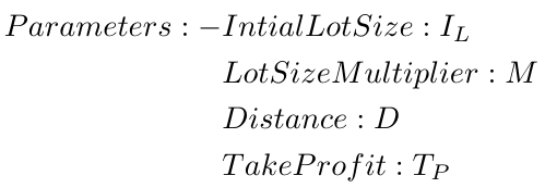
Let's first take a look at the parameters we will be optimizing i.e. parameters of the strategy.

Parameters of the Strategy:

1. Initial Position (IP): The Initial Position is a binary variable that sets the stage for the direction of our trading strategy. A value of 1 signifies a buy action, indicating that we are entering the market with the expectation of prices rising. Conversely, a value of 0 represents a sell action, suggesting that we anticipate a decline in prices. This initial choice may be a critical decision point, as it determines the overall bias of our trading strategy and sets the tone for subsequent actions. After the optimization we will know for sure which one is better to buy or sell.
2. Initial Lot Size (IL): The Initial Lot Size defines the magnitude of our first order within a trading cycle. It establishes the scale at which we will be participating in the market and lays the groundwork for the size of our subsequent transactions. Choosing an appropriate Initial Lot Size is crucial, as it directly impacts the potential profits and losses associated with our trades. It is essential to strike a balance between maximizing our potential returns and managing our risk exposure. It depends heavily on what lot size multiplier we choose, as if the multiplier is higher, this should be lower, otherwise the lot size of subsequent orders would explode quite quickly.
3. Distance (D): The Distance is a spatial parameter that determines the interval between the open price levels of our orders. It influences the entry points at which we will execute our trades and plays a significant role in defining the structure of our trading strategy. By adjusting the Distance parameter, we can control the spacing between our orders and optimize our entries based on market conditions and our risk tolerance.
4. Lot Size Multiplier (M): The Lot Size Multiplier is a dynamic factor that allows us to escalate the lot size of our subsequent orders based on the progression of the trading cycle. It introduces a level of adaptability to our strategy, enabling us to increase our exposure as the market moves in our favor or reduce it when faced with adverse conditions. By carefully selecting the Lot Size Multiplier, we can tailor our position sizing to capitalize on profitable opportunities while managing risk.
5. Number of Orders (N): The Number of Orders represents the total count of orders we will place within a single trading cycle/grid cycle. This is not exactly a parameter of the strategy, rather it is a parameter that we will take into account while optimizing the real parameters of the strategy.

It is crucial to have a firm grasp of the parameters that will be the focus of our optimization efforts. These parameters serve as the foundation upon which we will construct our strategy, and understanding their roles and implications is essential for making informed decisions and achieving our desired outcomes.

For simplicity, we present these parameters in their basic forms. However, it's important to note that in mathematical equations, some of these variables would be denoted using subscript notation to distinguish them from other variables.

These parameters serve as the foundation for constructing our profit function. The profit function is a mathematical representation of how our profit (or loss) is influenced by changes in these variables. It is a crucial component of our optimization process, enabling us to quantitatively assess the outcomes of various trading strategies under different scenarios.

With these parameters established, we can now proceed to define the components of our profit function:

Let's calculate the profit function for a simplified scenario where we choose to buy and have only two orders. We'll assume that the lot size multiplier is 1, meaning both orders have the same lot size of 0.01.

To find the profit function, we first need to determine the breakeven point. Let's assume we have two buy orders, B1 and B2. B1 is placed at price 0, and B2 is placed at a distance D below B1, i.e., at price -D. (Note that the negative price here is used for the sake of analysis and doesn't affect the outcome, as the analysis depends on the distance parameter D rather than the exact price levels.)

Now, let's say the breakeven point is at a distance x below B1. At this point, we will have a loss of -x pips from B1 and a profit of +x pips from B2.

If the lot sizes are equal (i.e., the lot size multiplier is 1), the breakeven point would be exactly in the middle of the two orders. However, if the lot sizes differ, we need to consider the lot size multiplier.

For example, if the lot size multiplier is 2 and the initial lot size is 0.01, then B1 will have a lot size of 0.01, and B2 will have a lot size of 0.02.

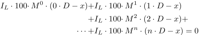
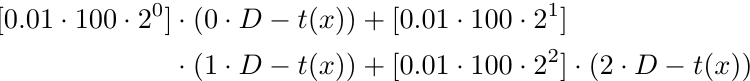
To find the breakeven point in this case, we need to find the value of x by solving the following equation:

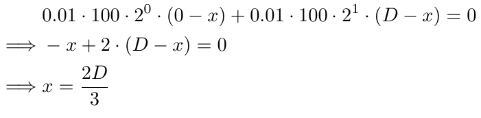
Let's analyze the components of the equation. The initial lot size, 0.01, is repeated in each part of the equation (the second part refers to the portion after the + sign). We multiply this by 100 to convert the lot size to an integer, and because we apply this conversion consistently throughout the equations, it maintains its significance. Next, we multiply it by 2^0 in the first part and 2^1 in the second part. These terms represent the lot size multiplier, with the power starting at 0 for the initial lot size and incrementing by 1 for each subsequent order. Finally, we use (0-x) in the first part, (D-x) in the second part, and ((i-1)D-x) in the i-th part because the i-th order is placed (i-1) times D pips below B1. Solving the equation for x yields 2D/3, meaning that the breakeven point lies 2D/3 pips below B1 (as defined by x in our equations). If D is 10, the breakeven would be 6.67 pips below B1, or 3.34 pips above B2. This price level is more likely to be reached compared to the breakeven at B1 (if we only had one order). This is the core concept behind the Griding Strategy: backing up previous orders until a profit is achieved.

Now, let's consider a case with 3 orders.

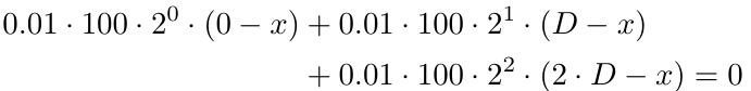
For 3 orders, we follow the same approach. The explanation for the 1st and 2nd parts remains the same. In the 3rd part, there are two changes: the power of 2 is incremented by 1, and D is now multiplied by 2. Everything else remains unchanged.

Solving for x further,

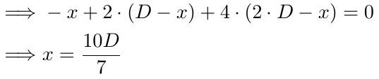
In the 3-order case, we find that the breakeven occurs when the price reaches 10D/7 pips below B1. If D is 10, the breakeven price would be 14.28 pips below B1, 4.28 pips below B2, and 5.72 pips above B3. Again, the price is more likely to reach this point compared to the breakeven at B1 (with 1 order) or the previous breakeven point. The breakeven continues to move lower, increasing the likelihood of the price reaching it, effectively backing up our previous orders if the price moves against us.

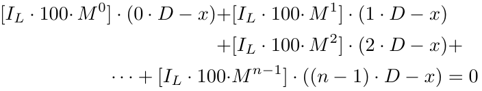
Let's generalize the formula for n orders.

Note: We assume all positions are Buy orders. The analysis for Sell orders is symmetric, so we'll keep it simple.

However, it turns out that this generalization is incorrect.

The reason for this can be explained with a simple example. Let's take the initial lot size to be 0.01 and the multiplier to be 1.5. First, we open a position with a lot size of 0.01. Then, we open a second position with a lot size of 0.01 * 1.5 = 0.015. However, after rounding, it becomes 0.01, as the lot size must be a multiple of 0.01. There are two issues here:

1. The equation calculates based on opening a position with a lot size of 0.015, which is practically not possible. Instead, we open a position with a lot size of 0.01.
2. This point is not exactly a problem but rather something that must be noted. Let's consider the same example. The first order was 0.01, and the second order was also 0.01 for practicality reasons. What should the third order's lot size be? We multiply the lot size multiplier by the last order's lot size, but should we multiply 1.5 by 0.01 or 0.015? If we multiply by 0.01, we are stuck in a loop that renders the point of having a multiplier useless. So, we go with 0.015 * 1.5 = 0.0225, which practically becomes 0.02, and so on.

As stated above, the second point is not exactly a problem. Let's fix the first problem using the Greatest Integer Factor (GIF) or floor function in mathematics, which says that we simply remove the decimal part of any positive number (we won't go into detail for negative numbers as lot size cannot be negative). Notation: floor(.) or [.]. Examples: floor(1.5) = [1.5] = 1; floor(5.12334) = [5.12334] = 5; floor(2.25) = [2.25] = 2; floor(3.375) = [3.375] = 3.

where, [.] represents GIF, i.e., Greatest Integer Factor. Further solving, we get:

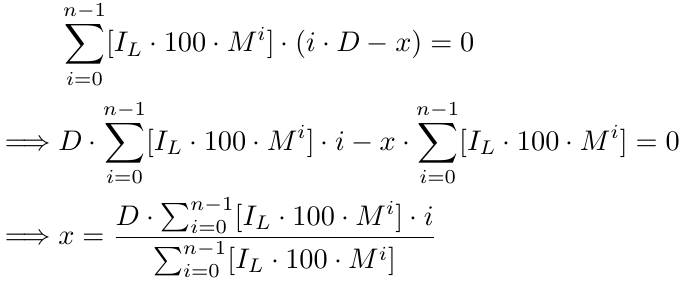
More formally, for x number of orders we have a break-even function b(x),

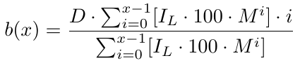
Now we have a breakeven function that gives us the breakeven price. It returns how many pips below B1 the breakeven price is. With the breakeven price, we need to determine the Take Profit (TP) level, which is simply TP pips above the b(x). Because b(x) is the B1 price level minus the breakeven price level, for the take profit level, we need to subtract TP from b(x). Thus, we have our take profit level, which we denote as t(x):

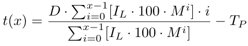
Given x, i.e., the number of orders, we have our take profit level. Now we need to calculate the profit given x. Let's try to find the profit function.

Assuming the price hits t(x), i.e., the take profit level, and the cycle closes, the profit/loss we receive from B1 is the price level of B1 minus t(x), with pips as the unit. A negative value means we have a loss, while a positive value shows that we have a profit. Similarly, the profit/loss we receive from B2 is the price level of B2 minus t(x), with pips as the unit, and we know that the B2 price level is exactly D pips below the B1 price level. For B3, the profit/loss is the price level of B3 minus t(x), with pips as the unit, and we know that the B3 price level is exactly 2 times D pips below the B1 price level. Note that we need to consider the initial lot size and lot size multiplier as well.

Mathematically, given x (i.e., the number of orders is 3), we have:

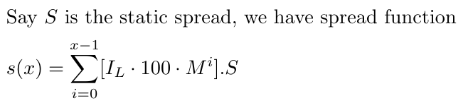
More formally, for x number of orders we have a profit function p(x),

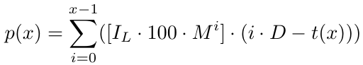
Let's understand what this means. Given any number of orders, assuming that the cycle closes in x number of orders (where "closes" means we hit the take profit level), we will have a profit given by the above equation p(x). Now that we have the profit function, let's try to calculate the cost function, which refers to the loss we will suffer if we lose a grid cycle with x number of orders (where "lost" means we can't open further orders to continue the grid cycle due to insufficient funds, as the grid strategy requires a lot of investments, or any other reason).

The cost function would look like this: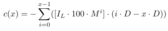

In this equation, the [.] part takes the Initial Lot Size and Lot Size Multiplier into account. The other part (i.D-x.D) considers x.D, which is the distance between the B1 price level and D pips below the order with the lowest price. We use x.D because that is precisely where we open a new order. If, for some reason, most likely insufficient funds, we fail to continue the cycle, that is the exact point at which we can say with certainty that we could not continue the cycle if we can't open the order at that price level (when the price reaches there). In essence, when we know for certain that we have failed to continue the cycle, the price level would be x.D pips below the B1 price level. As a result, we will have a loss of (0.D-x.D) from the B1 order, (1.D-x.D) from the B2 order, and so on until the last order, which is the Bx order, from which we will have a loss of ((x-1).D-x.D)=-D. This makes sense because we are D pips below the last order (the order with the lowest price level).

More formally, for x number of orders we have a cost function c(x),

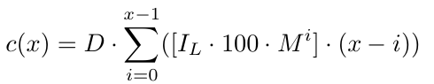
We also need to consider the spread, which we will assume to be a constant spread for simplicity, as taking a dynamic spread would be quite complex. Let's say S is the static spread, which we will keep equal to 1-1.5 for EURUSD. The spread may change depending on the currency pair, but this strategy will work best with currencies that have lower volatility, like EURUSD.

It's important to note that our adjustment takes into account all trades, from zero to x-1, recognizing that the spread affects every trade, whether profitable or not. For simplicity, we're currently treating the spread (denoted as S) as a constant value. This decision is made to avoid complicating our mathematical analysis with the added variability of a fluctuating spread. Although this simplification limits the realism of our model, it allows us to focus on the core aspects of our strategy without getting bogged down by excessive complexity.

Now that we have all the necessary functions, we can plot them in Desmos.

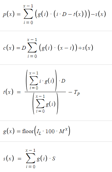
Given the above parameters, we have the following table, where changing x gives different values of p(x) and c(x):

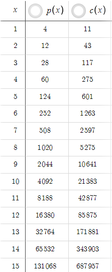
In this scenario, p(x) is always less than c(x), but this can easily be changed by increasing the TP. For example, if we increase the TP from 5 to 50:

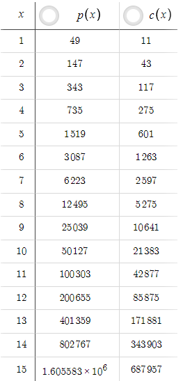
Now, p(x) is always greater than c(x). A novice trader might think that if we can get such high levels of risk-reward ratio with TP=50, why keep TP=5? However, we must take probability into account. The increment of TP from 5 to 50 has drastically decreased the probability of the price reaching the take profit level. We have to realize that there is no point in having a good risk-reward ratio if we never or very rarely hit the take profit. To account for probabilities, we need price data and coding-based optimization rather than just equations, which we will explore in further parts of the series.

You can use this Desmos Graph Link to see the plot of these functions and play with the parameters to gain a better understanding of this strategy.

With that, we have completed the Mathematical Part of the Optimization. In the next sections, we will delve deeper into the practical aspects of implementing this strategy, considering real-world market conditions and the challenges that come with them. By combining the mathematical foundation we have established here with data-driven analysis and optimization techniques, we can refine the grid trading strategy to better suit our needs and maximize its potential for profitability.

Final Thoughts: As mentioned earlier, numerous parameters indicate a high potential for profit. However, it's crucial to understand that these figures serve primarily as illustrations. The reason behind this is the absence of a vital component in mathematical optimization: probability. Incorporating probability into our mathematical model is a complex task, but it's an indispensable factor that cannot be ignored. To address this, we will conduct simulations on price data, allowing us to consider probability in our calculations and improve the accuracy of our model.

Simulating Calculations in Python

In this simulation, we will calculate and plot p(x) and c(x) against x, where x represents the number of orders. The values of p(x) and c(x) will be plotted on the y-axis, while x will be on the x-axis. This visualization will provide quick insights into the changes in p(x) and c(x), and help identify which function is greater at different points. Additionally, we will generate a table that displays the exact values of p(x) and c(x) for each x, as these values might not be easily readable from the plot alone. This combination of the plot and the table will offer a comprehensive understanding of the behavior of p(x) and c(x).

Python Code:

import numpy as np
import matplotlib.pyplot as plt
from matplotlib.ticker import FuncFormatter

# Parameters
D = 10     # Distance
I_L = 0.01 # Initial Lot Size
M = 2      # Lot Size Multiplier
S = 1      # Spread
T_P = 50   # Take Profit

# Values of x to evaluate
x_values = range(1, 21)  # x from 1 to 20

def g(x, I_L, M):
    return np.floor(I_L * 100 * M ** x)

def s(x, I_L, M, S):
    return sum(g(i, I_L, M) * S for i in range(x))

def t(x, D, I_L, M, T_P):
    numerator = sum(i * g(i, I_L, M) for i in range(x)) * D
    denominator = sum(g(i, I_L, M) for i in range(x))
    return (numerator / denominator) - T_P

def p(x, D, I_L, M, S, T_P):
    return sum(g(i, I_L, M) * (i * D - t(x, D, I_L, M, T_P)) for i in range(x)) - s(x, I_L, M, S)

def c(x, D, I_L, M, S):
    return D * sum(g(i, I_L, M) * (x - i) for i in range(x)) + s(x, I_L, M, S)

# Calculate p(x) and c(x) for each x
p_values = [p(x, D, I_L, M, S, T_P) for x in x_values]
c_values = [c(x, D, I_L, M, S) for x in x_values]

# Formatter to avoid exponential notation
def format_func(value, tick_number):
    return f'{value:.2f}'

# Plotting
fig, axs = plt.subplots(2, 1, figsize=(12, 12))

# Combined plot for p(x) and c(x)
axs[0].plot(x_values, p_values, label='p(x)', marker='o')
axs[0].plot(x_values, c_values, label='c(x)', marker='o', color='orange')
axs[0].set_title('p(x) and c(x) vs x')
axs[0].set_xlabel('x')
axs[0].set_ylabel('Values')
axs[0].set_xticks(x_values)
axs[0].grid(True)
axs[0].legend()
axs[0].yaxis.set_major_formatter(FuncFormatter(format_func))

# Create table data
table_data = [['x', 'p(x)', 'c(x)']] + [[x, f'{p_val:.2f}', f'{c_val:.2f}'] for x, p_val, c_val in zip(x_values, p_values, c_values)]

# Plot table
axs[1].axis('tight')
axs[1].axis('off')
table = axs[1].table(cellText=table_data, cellLoc='center', loc='center')
table.auto_set_font_size(False)
table.set_fontsize(10)
table.scale(1.2, 1.2)

plt.tight_layout()
plt.show()

Code Explanation:

1. Import Libraries:

   • numpy is imported as np for numerical operations.
   • matplotlib.pyplot is imported as plt for plotting.
   • FuncFormatter is imported from matplotlib.ticker to format axis tick labels.

2. Set Parameters:

   • Define constants D, I_L, M, S, and T_P which represent Distance, Initial Lot Size, Lot Size Multiplier, Spread, and Take Profit, respectively.

3. Define Range for x:

   • x_values is set to a range of integers from 1 to 20.

4. Define Functions:

   • g(x, I_L, M): Calculates the value of g based on the given formula.
   • s(x, I_L, M, S): Calculates the sum of g(i, I_L, M) * S for i from 0 to x-1 .
   • t(x, D, I_L, M, T_P): Calculates the value of t based on the given formula, using a numerator and denominator.
   • p(x, D, I_L, M, S, T_P): Calculates p(x) using the given formula.
   • c(x, D, I_L, M, S): Calculates c(x) using the given formula.

5. Calculate p(x) and c(x) Values:

   • p_values is a list of p(x) for each x in x_values.
   • c_values is a list of c(x) for each x in x_values.

6. Define Formatter:

   • format_func(value, tick_number): Defines a formatter function to format y-axis tick labels to two decimal places.

7. Plotting:

   • fig, axs = plt.subplots(2, 1, figsize=(12, 12)) : Creates a figure and two subplots arranged in a single column.

   First Subplot (Combined Plot for p(x) and c(x)):

   • axs[0].plot(x_values, p_values, label='p(x)', marker='o'): Plots p(x) against x with markers.
   • axs[0].plot(x_values, c_values, label='c(x)', marker='o', color='orange'): Plots c(x) against x with markers in orange color.
   • axs[0].set_title('p(x) and c(x) vs x'): Sets the title of the first subplot.
   • axs[0].set_xlabel('x'): Sets the x-axis label.
   • axs[0].set_ylabel('Values'): Sets the y-axis label.
   • axs[0].set_xticks(x_values): Ensures x-axis ticks are displayed for each x value.
   • axs[0].grid(True): Adds a grid to the plot.
   • axs[0].legend(): Displays the legend.
   • axs[0].yaxis.set_major_formatter(FuncFormatter(format_func)): Applies the formatter to the y-axis to avoid exponential notation.

   Second Subplot (Table):

   • table_data: Prepares table data with columns x , p(x) , and c(x) , and their corresponding values.
   • axs[1].axis('tight'): Adjusts the subplot axis to tightly fit the table.
   • axs[1].axis('off'): Turns off the axis for the table subplot.
   • table = axs[1].table(cellText=table_data, cellLoc='center', loc='center'): Creates a table in the second subplot with centered cell text.
   • table.auto_set_font_size(False): Disables automatic font size adjustment.
   • table.set_fontsize(10): Sets the font size of the table.
   • table.scale(1.2, 1.2): Scales the table size.

8. Layout and Display:

   • plt.tight_layout(): Adjusts the layout to prevent overlapping.
   • plt.show(): Displays the plots and table.

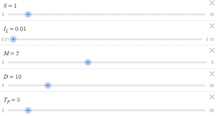
We have used the following default parameters (can be easily changed to see the different results):

# Parameters
D = 10     # Distance
I_L = 0.01 # Initial Lot Size
M = 2      # Lot Size Multiplier
S = 1      # Spread
T_P = 50   # Take Profit

Result:

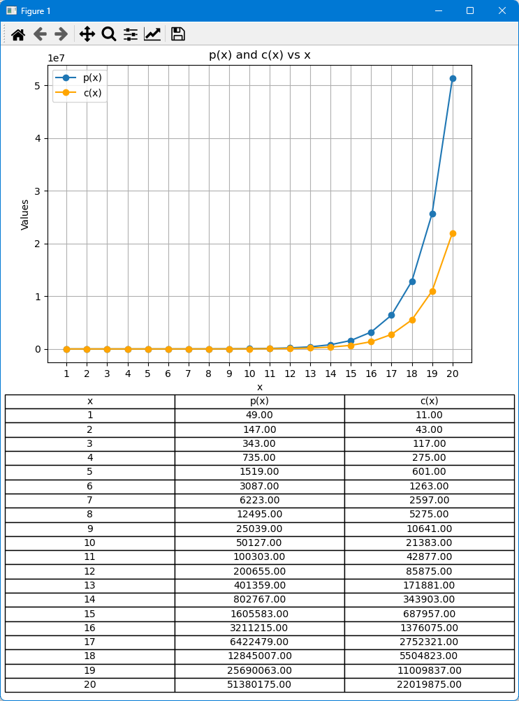
Note: A Python file containing the code discussed above has been attached at the bottom of the article.

Conclusion

In the fourth installment of our series, we focused on optimizing the Simple Grid strategy through mathematical analysis and the role of probability, which is often overlooked in grid and hedging strategies. Future articles will transition from theory to practical, code-based applications, applying our insights to real trading scenarios to help traders enhance returns and manage risks effectively. We appreciate your continued feedback and encourage further interaction as we explore, refine, and succeed in trading strategies together.

Happy Coding! Happy Trading!