Measuring Indicator Information

Introduction

Machine learning relies on training data to learn the general behaviour of the market to ultimately make fairly accurate predictions. The chosen learning algorithm has to wade through a carefully selected sample to extract meaningful information . The reason why many fail to successfully apply these sophiscated tools is because, most of the meaningful information is hidden in noisy data. It may not be apparent to many strategy developers that the data sets we use may not be appropriate for model training.

Indicators can be thought of as purveyors of information about the underlying price series they are applied to. Using this premise, entropy can be used to measure how much information is communicated by an indicator. Using steps and tools documented in the book, Testing and Tuning Market Trading Systems (TTMTS)  written by Timothy Masters, we will demonstrate how these can be used to evaluate the structure of indicator data.

Why measure Indicator Information

Often when using  machine learning tools for strategy development we resort to simply throwing all sorts of data at the  algorithms with the hope that something will come of it. Ultimately success will depend on the quality of the predictor(s) used in the model and effective predictors usually have cetain characteristics. One of them being laden with significant information content.

The amount of information in variables used for model training  is important but is not the only requirement for effective model training. Therefore, measuring infomation content can be used to screen indicators that would otherwise be blindly used during the training process.  This is where the concept of entropy is applied.

Entropy

Entropy has been written about a number of times already on MQL5.com. I apologize to the reader as they will have to endure another definition, but i promise this is essential to understanding the concept's application. Previous articles have provided the history and derivation of the entropy calculation so for the sake of brevity we will begin with the equation.

                                                        

H(X) means the entropy of X, X is a discrete variable representing an arbitrary variable, say a message. The contents of the message can only assume a finite number of values. This is represented in the equation as small x. Small x are the observed values of the messages, such that, if all the possible values of x were enumerated in a set, N.

Consider an example of a fair dice. The dice, when rolled, can be perceived as providing information, that determines the outcome of a game. The dice has 6 unique sides numbered 1 to 6. The probability of observing anyone of the numbers facing up is 1/6.

Using this example, Big X would be the dice and small x could be any of the numbers painted on the sides of dice. All of which are placed in set N ={ 1,2,3,4,5,6}. Applying the formula  the entropy of this dice is 0.7781.

                                                         

Now consider another dice, which has a manufacturing defect. It has 2 sides with the same number painted on it. For this defective dice the set N of possible values is  {1,1,3,4,5,6}. Using the formula again we get an average entropy value of 0.6778  .

                                                 

Comparing the values  we notice that the information content has decreased. Analyzing  both die , when the probabilities for observing each possible value are all equal then the entropy equation produces its greatest possible value. Therefore the entropy  reaches its maximum average when the probabilities of all the possible values are equal.

If we discard the defective dice for an indicator that produces traditional real numbers as output. Then, X becomes the indicator and small x will be the range of values that the indicator can assume. Before proceeding further we have a problem because the entropy equation deals strictly with discrete variables. Transforming the equation to work with continuous variables is possible but the application of such would be difficult , so it is easier to stick to the realm of discrete numbers.

Calculating the entropy of an indicator

To apply the equation of entropy  to continous variables we have to discretize the values of the indicator.This is done by dividing the range of values into intervals of equal size, then counting the number of values that fall into each interval. Using this method the original set that enumerated the maximum range of all values of the indicator is replaced by subsets , each of which are the selected intervals.

When dealing with continuous variables the variation in probabilities of the possible values that can be assumed by the variable becomes significant as it provides an import facet to the application of entropy to indicators.

Going back to the first example of the dice. If we divide the final entropy values of each by the log(N) for each ones respective n. The first die produces 1, whilst the defective die results in 0.87. Dividing the entropy value by the log of the number of values the variable can assume produces a measure that is relative to the variable's theoretical maximum entropy. Referred to as proportional or relative entropy.

It is this value that would be useful in our assessment of indicators as it will point to how close the entropy of the indicator is to its theoretical maximum average. The closer it is to one, the maximum, the better and anything on the other end may hint at an indicator that would be a poor candidate for use in any kind of machine learning endeavour. 

                                  

The final equation that will be applied shown above and the code is implemented below as a mql5 script which is available for download as an attachement at the end of the article. Using the script we will be able to analyze most indicators.

A script for calculating the entropy of an indicator

The Script is invoked with the following user adjustable parameters:

• TimeFrame - selected timeframe to analyze indicator values on.
• IndicatorType - Here the user can select one of the built in indicators for analysis. To specify a custom indicator , select Custom indicator option and input the indicator's name in the next parameter value.
  
• CustomIndicatorName - If Custom indicator option selected for the prior parameter , the user has to input the correct name of the indicator here.
  
• UseDefaults - If set to true the default user inputs hard coded into the indicator will be used.
  
• IndicatorParameterTypes - this is comma delimited  string that lists the data types of the indicator in the right order - An example of  possible input, assuming  indicator to be analyzed accepts 4 inputs of type double , integer, integer, string respectively, user simply has to input "double , integer, integer, string " , the short form "d , i, i, s " is supported as well where d= double , i=integer and s=string. Enum values are mapped to the integer type.
  
• IndicatorParameterValues - Like the prior input, this also a comma delimited list of values, for example , using the previous example, "0.5,4,5,string_value". If there is any error in the formating of the parameters for either of IndicatorParameterValues or IndicatorParameterTypes, will result in indicator's  default values being used for any specific values that cannot be deciphered or is missing.
  Check the experts tab for error messages. Note that there is no need include the name of the indicator here, if a custom indicator is being considered, it must be specified by CustomIndicatorName.
• IndicatorBuffer - The user can stipulate which of the indicator buffers to analyze.
  
• HistoryStart - The start date of the history sample.
  
• HistorySize - This the number of bars to analyze relative to HistoryStart.
  
• Intervals - This parameter is used indicate the number intervals that will be created for the the descretization process. The author of TTMTS specifies 20 intervals for a sample size of several thousand with 2 stipulated as a hard minimum value.  I have added  my own spin on a appropriate  value to use here by implementing the possibility to vary the number of intervals relative to the sample size, specifically 51 for every 1000 samples. This option is available if a user inputs any value less that 2. So, to be clear setting Interval to any number less than 2 and the number of intervals used will change according to the number of bars being analyzed.
  

//--- input parameters
input ENUM_TIMEFRAMES Timeframe=0;
input ENUM_INDICATOR  IndicatorType=IND_BEARS;
input string   CustomIndicatorName="";
input bool     UseDefaults=true;
input string   IndicatorParameterTypes="";
input string   IndicatorParameterValues="";
input int      IndicatorBuffer=0;
input datetime HistoryStart=D'2023.02.01 04:00';
input int HistorySize=50000;
input int      Intervals=0;

int handle=INVALID_HANDLE;
double buffer[];
MqlParam b_params[];
//+------------------------------------------------------------------+
//| Script program start function                                    |
//+------------------------------------------------------------------+
void OnStart()
  {
   if(!processParameters(UseDefaults,b_params))
      return;

   int y=10;
   while(handle==INVALID_HANDLE && y>=0)
     {
      y--;
      handle=IndicatorCreate(Symbol(),Timeframe,IndicatorType,ArraySize(b_params),b_params);
     }
//---
   if(handle==INVALID_HANDLE)
     {
      Print("Invalid indicator handle, error code: ",GetLastError());
      return;
     }

   ResetLastError();
//---
   if(CopyBuffer(handle,IndicatorBuffer,HistoryStart,HistorySize,buffer)<0)
     {
      Print("error copying to buffer, returned error is ",GetLastError());
      IndicatorRelease(handle);
      return;
     }
//---
   Print("Entropy of ",(IndicatorType==IND_CUSTOM)?CustomIndicatorName:EnumToString(IndicatorType)," is ",relativeEntroy(Intervals,buffer));
//---
   IndicatorRelease(handle);
  }
//+------------------------------------------------------------------+

//+------------------------------------------------------------------+
//|                                                                  |
//+------------------------------------------------------------------+
bool processParameters(bool use_defaults,MqlParam &params[])
  {

   bool custom=(IndicatorType==IND_CUSTOM);

   string ind_v[],ind_t[];

   int types,values;

   if(use_defaults)
      types=values=0;
   else
     {
      types=StringSplit(IndicatorParameterTypes,StringGetCharacter(",",0),ind_t);
      values=StringSplit(IndicatorParameterValues,StringGetCharacter(",",0),ind_v);
     }

   int p_size=MathMin(types,values);

   int values_to_input=ArrayResize(params,(custom)?p_size+1:p_size);

   if(custom)
     {
      params[0].type=TYPE_STRING;
      params[0].string_value=CustomIndicatorName;
     }

//if(!p_size)
//  return true;

   if(use_defaults)
      return true;

   int i,z;
   int max=(custom)?values_to_input-1:values_to_input;

   for(i=0,z=(custom)?i+1:i; i<max; i++,z++)
     {
      if(ind_t[i]=="" || ind_v[i]=="")
        {
         Print("Warning: Encountered empty string value, avoid adding comma at end of string parameters");
         break;
        }

      params[z].type=EnumType(ind_t[i]);

      switch(params[z].type)
        {
         case TYPE_INT:
            params[z].integer_value=StringToInteger(ind_v[i]);
            break;
         case TYPE_DOUBLE:
            params[z].double_value=StringToDouble(ind_v[i]);
            break;
         case TYPE_STRING:
            params[z].string_value=ind_v[i];
            break;
         default:
            Print("Error: Unknown specified parameter type");
            break;
        }
     }

   return true;

  }


//+------------------------------------------------------------------+
//|                                                                  |
//+------------------------------------------------------------------+
ENUM_DATATYPE EnumType(string type)
  {
   StringToLower(type);
   const ushort firstletter=StringGetCharacter(type,0);

   switch(firstletter)
     {
      case 105:
         return TYPE_INT;
      case 100:
         return TYPE_DOUBLE;
      case 115:
         return TYPE_STRING;
      default:
         Print("Error: could not parse string to match data type");
         return ENUM_DATATYPE(-1);
     }

   return ENUM_DATATYPE(-1);
  }
//+------------------------------------------------------------------+

Just a note on the value selected for Intervals: Changing the number of intervals used in the calculation will vary the final entropy value. When conducting analysis it would be wise to have some consistency so as to minimize the effects of the independent input used. In the script the relative entropy calculation is encapsulated in a function defined in the Entropy.mqh file.

The script simply prints the resulting entropy value in the experts tab. Running the script for various built in and custom indicators yields the results shown below. Its interesting to note William's Percent Range  has relative entropy close to perfection. Compare it with the Market Facilitation Index indicator which shows a dissapointing result.

With these results we can take further steps to process the data to make it amenable for machine learning algorithms. This involves conducting rigorous analysis of the statistical properties of the indicator. Studying a distribution of the indicator values will reveal any problems with skew and outliers. All of which can degrade model training.

As an example we examine some statistical properties of two indicators analyzed above.

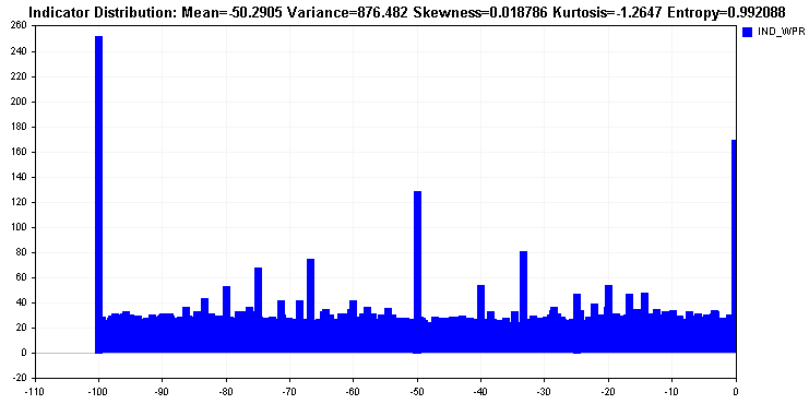
The distribution of Williams's percent range reveals how almost all the values are spread across the entire range, apart from being multi modal the distribution is fairly uniform. Such a distribution is ideal and is reflected in the entropy value.

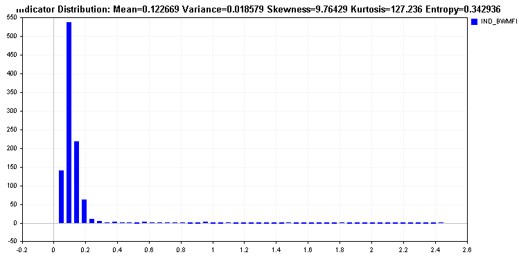
This is in contrast to the Market Facilitation Index distribution which has a  long tail. Such an indicator would be problematic for most learning algorithms and requires transformation of the values. Transforming the values should lead to an improvement in indicator's relative entropy.

Improving the information content of an indicator

It should be stated that alterations that boost indicator entropy should not be seen as a way to improve the accuracy of signals provided by the indicator. Boosting entropy will not turn a useless indicator into the holygrail. Improving entropy is about processing the indicator data for effective use in predictive models .

This option should be considered when the entropy value is hopelessly bad, anything well below 0.5 and closer to zero. Upperbound thresholds are purely abitrary. It is up to the developer to pick an acceptable minimum value. The whole point is to produce a distribution of indicator values that is as close to uniform as possible. The decision to apply a transformation should be based on analysis conducted on a sizeable and representative sample of indicator values.

The transformation applied should not alter the undelying behaviour of the indicator. The transformed indicator should have a similar shape as the raw indicator , for example the location of troughs and  peaks should be similar in both series. If this is not the case then we risk losing potentially useful information.

There are numerous methods of transformation that target different aspects of test data imperfections. We will only consider a few simple transformations that look to fix obvious defects revealed through basic statistical analysis. Preprocessing is a vast branch of machine learning. Anyone who hopes to master the application of machine learning methods is advised to gain more knowledge in this field.

To illustrate the effect of some transformations, we present a script that has the option to apply various transformations and also displays the distribution of the data being analyzed. The script implements 6 examples of transformation functions:

• the square root function transform is appropriate for squashing occasional indicator values that deviate considerably from the majority.

• the cube root transform is another squashing function that is best applied indicators with negative values.

• whilst the log transform compresses values to a larger extent than previously mentioned compressing transformations.

• the hyperbolic tangent and logistic transforms should be applied on data values of a suitable scale to avoid problems of producing invalid numbers (nan errors).

• the extreme transform induces extreme uniformity in a data set. It should be applied only to indicators that produce mostly unique values with very few similar figures.

A script to compare transformed indicator values

Compared to the earlier script it contains  the same user inputs  to specify the indicator to be analyzed. The new  inputs are described below:

• DisplayTime - the script displays a graphic of the distribution of the indicator. DisplayTime is an integer value in seconds, which is the amount of time the graphic will be visible before being removed.

• ApplyTransfrom - is a boolean value that sets the mode for the script. When false the script draws the distribution and displays basic statistics of the sample along with the relative entropy. If true is set, it applies a transformation on the raw indicator values and displays the relative entropy values before and after transformation. The distribution of the modified samples with also be drawn as a curve in red.

• Select_transform - is an enumeration providing the transforms described earlier that can be applied    to possibly boost the entropy of the indicator.

//+------------------------------------------------------------------+
//|                                            IndicatorAnalysis.mq5 |
//|                        Copyright 2023, MetaQuotes Software Corp. |
//|                                             https://www.mql5.com |
//+------------------------------------------------------------------+
#property copyright "Copyright 2023, MetaQuotes Software Corp."
#property link      "https://www.mql5.com"
#property version   "1.00"
#property script_show_inputs
#include<Entropy.mqh>
//--- input parameters
input ENUM_TIMEFRAMES Timeframe=0;
input ENUM_INDICATOR  IndicatorType=IND_CUSTOM;
input string   CustomIndicatorName="";
input bool     UseDefaults=false;
input string   IndicatorParameterTypes="";
input string   IndicatorParameterValues="";
input int      IndicatorBuffer=0;
input datetime HistoryStart=D'2023.02.01 04:00';;
input int HistorySize=50000;
input int DisplayTime=30;//secs to keep graphic visible
input bool ApplyTransform=true;
input ENUM_TRANSFORM Select_transform=TRANSFORM_LOG;//Select function transform

int handle=INVALID_HANDLE;
double buffer[];
MqlParam b_params[];
//+------------------------------------------------------------------+
//| Script program start function                                    |
//+------------------------------------------------------------------+
void OnStart()
  {
//---
   if(!processParameters(UseDefaults,b_params))
      return;

   int y=10;
   while(handle==INVALID_HANDLE && y>=0)
     {
      y--;
      handle=IndicatorCreate(_Symbol,Timeframe,IndicatorType,ArraySize(b_params),b_params);
     }
//---
   if(handle==INVALID_HANDLE)
     {
      Print("Invalid indicator handle, error code: ",GetLastError());
      return;
     }

   ResetLastError();
//---
   if(CopyBuffer(handle,IndicatorBuffer,HistoryStart,HistorySize,buffer)<0)
     {
      Print("error copying to buffer, returned error is ",GetLastError());
      IndicatorRelease(handle);
      return;
     }
//---
   DrawIndicatorDistribution(DisplayTime,ApplyTransform,Select_transform,IndicatorType==IND_CUSTOM?CustomIndicatorName:EnumToString(IndicatorType),buffer);
//---
   IndicatorRelease(handle);
  }
//+------------------------------------------------------------------+
bool processParameters(bool use_defaults,MqlParam &params[])
  {

   bool custom=(IndicatorType==IND_CUSTOM);

   string ind_v[],ind_t[];

   int types,values;

   if(use_defaults)
      types=values=0;
   else
     {
      types=StringSplit(IndicatorParameterTypes,StringGetCharacter(",",0),ind_t);
      values=StringSplit(IndicatorParameterValues,StringGetCharacter(",",0),ind_v);
     }

   int p_size=MathMin(types,values);

   int values_to_input=ArrayResize(params,(custom)?p_size+1:p_size);

   if(custom)
     {
      params[0].type=TYPE_STRING;
      params[0].string_value=CustomIndicatorName;
     }

   if(use_defaults)
      return true;

   int i,z;
   int max=(custom)?values_to_input-1:values_to_input;

   for(i=0,z=(custom)?i+1:i; i<max; i++,z++)
     {
      if(ind_t[i]=="" || ind_v[i]=="")
        {
         Print("Warning: Encountered empty string value, avoid adding comma at end of string parameters");
         break;
        }

      params[z].type=EnumType(ind_t[i]);

      switch(params[z].type)
        {
         case TYPE_INT:
            params[z].integer_value=StringToInteger(ind_v[i]);
            break;
         case TYPE_DOUBLE:
            params[z].double_value=StringToDouble(ind_v[i]);
            break;
         case TYPE_STRING:
            params[z].string_value=ind_v[i];
            break;
         default:
            Print("Error: Unknown specified parameter type");
            break;
        }
     }

   return true;

  }


//+------------------------------------------------------------------+
//|                                                                  |
//+------------------------------------------------------------------+
ENUM_DATATYPE EnumType(string type)
  {
   StringToLower(type);
   const ushort firstletter=StringGetCharacter(type,0);

   switch(firstletter)
     {
      case 105:
         return TYPE_INT;
      case 100:
         return TYPE_DOUBLE;
      case 115:
         return TYPE_STRING;
      default:
         Print("Error: could not parse string to match data type");
         return ENUM_DATATYPE(-1);
     }

   return ENUM_DATATYPE(-1);
  }
//+------------------------------------------------------------------+

Continuing with the examples we compare application of both square root  and cube root transforms.

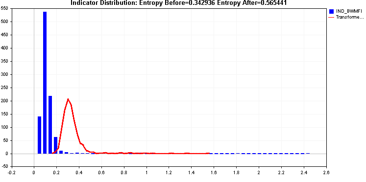
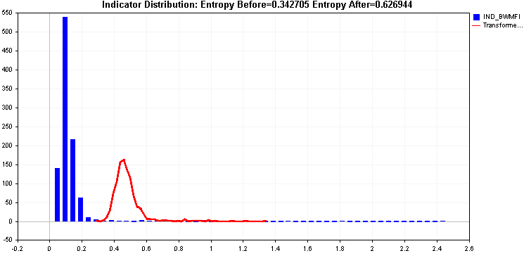
Both provide an improvement in entropy but that right tail could be problematic, the two transforms applied so far have not been able to deal with it effectively.

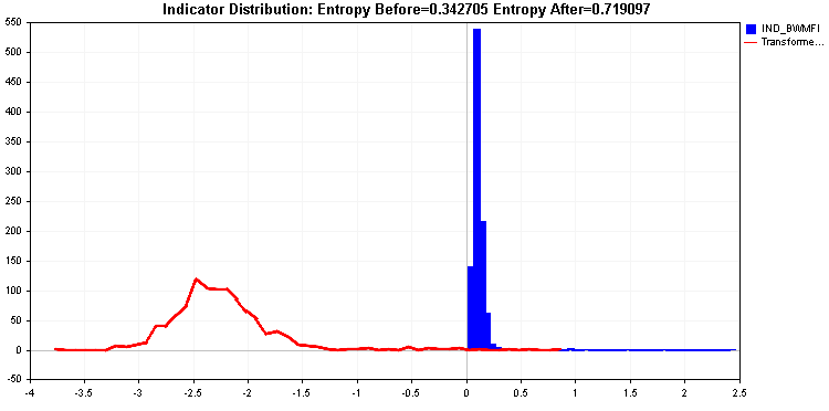
The log transform produces an even better entropy value. Still the tails are quite significant. As a last resort we can apply the extreme transform.

Conclusion

We explored the concept of entropy to evaluate the need for indicator values to be transformed before being used in predictive model training.

The concept was implemented in two scripts. Namely EntropyIndicatorAnalyis which prints the relative entropy of a sample in the experts tab. The other script IndicatorAnalysis goes one step further by drawing the distribution of the raw and transformed indicator values along with displaying the before and after relative entropy values.

Whilst the tools may be useful it should be noted they cannot be applied to all kinds of indicators. Generally, arrow based indicators that contain empty values would not be appropriate for the scripts described here. In such cases other encoding techniques would be necessary.

The topic of data transformation is only a subset of possible preprocessing steps that should be considered when building any kind of predictive model. Using such techniques will help in extracting truly unique relationships that could provide the edge needed to beat the markets.

File name	Description
Mql5/Include/Entropy.mqh	include file that contains various definitions for functions used to calculate entropy and also utility functions used by the scripts attached.
Mql5/Scripts/IndicatorAnalysis.mq5	a script that displays a graphic showing the distribution of indicator values, along with its entropy.
Mql5/Scripts/EntropyIndicatorAnalysis	a script that can be used to calculate the entropy of an indicator