MQL5 Wizard Techniques you should know (Part 79): Using Gator Oscillator and Accumulation/Distribution Oscillator with Supervised Learning

Introduction

In our last 2 articles, we tested, as usual, ten signal patterns while using the indicator pairing of the Gator oscillator and Accumulation/Distribution oscillator. In doing so, as has been our practice, we found three consistent laggard patterns: 0, 3, and 4. Rather than discard or disregard these, this article aims to explore whether supervised learning can revive their performance. We employ a CNN enhanced with kernel regression and dot product similarity and examine if networks with such architecture can extract hidden value from signals that sometimes initially appear weak. As per the last two articles all testing is on the pair GBP JPY and on the 30 minute time frame.

Kernel Regression with Dot Product Similarity

Our choice for a supervised learning model is a CNN that uses kernel regression and dot product similarity. Kernel regression estimates the outputs of each layer in a CNN by weighting the observed inputs in accordance to their similarity to a specific query point. This similarity is quantified using the dot product similarity as the kernel function. In our model, whose code is shared below in the next section, the _dot_product_kernel_regression method works out the similarity between all time positions in a feature map using the function torch.bmm(x, x.T) to which we add softmax normalization that is quite similar to self attention.

The dot product’s role is to be a data-adaptive measure of similarity, where a high product means two positions have the same pattern of activation across channels, which can lead to a greater influence in the weighted sum. An analogy, or different way of looking at this, could be like giving each position “votes” proportional to its agreement with the query position. A CNN layer can be thought of as a spreadsheet where the rows are time steps and the columns are features. In this setting, a single row is taken to represent a ‘position’. The ‘query position’ is therefore the current row that is being updated. In the process of performing these updates, comparisons are made between it and every other position to quantify how similar they are. These updates take place in Backpropagation.

Mathematically, new weights could be defined as follows. Given feature vectors xi​ and xj, the weight wij is:

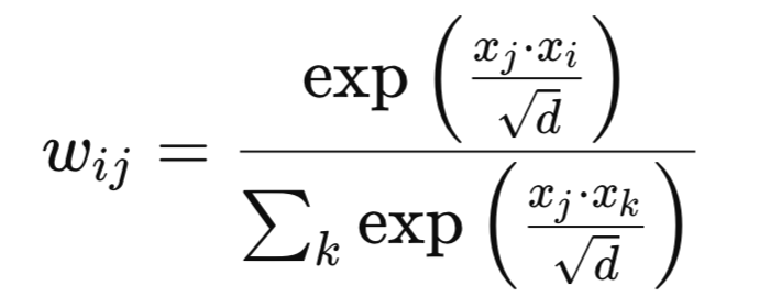
Where:

• d - is the channel dimension.
• exp - is the natural logarithm

Our weigh matrix performs a non-local smoothing across the sequence that is not restricted to neighboring positions like in a convolution. The effect of this is that it is able to capture long-range dependencies and correlations within the feature space, potentially boosting performance in time series and structures data tasks. For guidance, the dot-product-similarity should be engaged when the task at hand exhibits meaningful correlations between non-adjacent features; and you want as attention-like mechanism that does not necessitate adding query/key/value projections. This can be particularly synergistic with CNNs since they capture local features and kernel regression, which adds global context.

Case for Guiding a CNN’s Kernel and Channel Sizes with Dot-Product

The dot product kernel regression exposes where and at what resolution correlations are strongest. Adjusting the CNN kernel sizes and channel depths, in step with a similarity structure, can do two things. Firstly, it can help match receptive fields to correlation length. This is especially the case in larger kernels if high similarity is able to persist over wide distances. Secondly, it can allocate channels in line with correlation complexity. More channels are allotted when similarity patterns vary strongly, and fewer when there is more uniformity. This has the potential to lead to an architecture that is both data-driven and task-specific, as opposed to fixed heuristics.

In our implementation of this, as shown in the source code in the following sections, the kernel sizes cycle through [3,5,7,9] while the channel depths also increase from 32 to 320. Every other layer applies a dot product regression, implying that the layers ‘see’ global correlation maps. If the similarity maps show broad peaks of larger kernels in the subsequent convolution layers, this can be leveraged. If the map shows sharp peaks, smaller kernels can be sufficient, and this would lead to focusing on small refinements. This can be akin to adaptive receptive field tuning guided by a global correlation signal.

When using in CNNs, one should consider running a pre-analysis where data is fed through a small CNN plus dot product kernel block in order to analyze correlation lengths, which can then serve as a basis for setting the main CNN’s kernel/ channel plan. Also, pairing early layers with smaller kernels when performing local edge/pattern detection should be preferred, with later layer kernel sizes then being guided by the observed similarity spread.

Possible Drawbacks and Possible Alternatives

Our premiere drawback/ disadvantage of using the dot product kernel the way we are should come as no surprise, and it is computation cost. Dot product similarity scales as O(L2) with a sequence length of L. This can be heavy for long signals or sizable feature inputs. Another concern is over-smoothing. If weights are too diffuse, features may become too homogeneous, thus resulting in a loss of some fine detail. Training instability is also another trouble spot. In large similarities, if there is no normalization, we can have cases of exploding weights. Finally, the memory overhead for storing a complete similarity matrix can have prohibitive costs. 

These concerns, though, do have some mitigation measures and these include using local-attention-windows. So instead of computing the similarity amongst all positions by exhausting the compute complexity formula already presented and linked above, we limit comparisons to a fixed window around each query position. This would cut compute/ memory and focus on blending the nearby relevant context. Besides this, we can also adopt temperature scaling. Here we simply multiply the similarity scores by 1/τ, the temperature. A lower temperature would lead to sharper, more selective weights where few positions/layer-rows dominate. A higher τ would yield smoother and more evenly distributed weights throughout the layer grids. The temperature would be an extra hyperparameter.

Finally, we can also use downsampling before performing the kernel regression. This would involve reducing the input data sequence length L by using pooling or stride convolutions prior to computing the dot product. Shorter L should speed up similarity calculations and also reduce memory requirements while still capturing large-scale correlations.

Alternative CNN Enhancements with the Dot-Product

Besides kernel regression with the dot product kernel, we can apply self-attention hybrid CNNs. With this we would use dot product regression as a non-local block alongside the CNN layers as opposed to a standard attention layer. This differs from our implementation, whose source is covered in the next section, in that in our model that we apply the kernel regression periodically in a convolutional stack. The hybrid would insert it in parallel branches and fuse outputs. We could also apply our kernel by multiscale feature fusion, where the kernel regression gets applied to features that are from several CNN layers and then get combined. The difference from what we have done is we are using kernel regression only at one layer at a time. Multiscale fusion merges global context from different layers/resolutions. 

We could have also applied the kernel by pretext tasks for regularization. In this scenario, we train the kernel regression outputs to solve auxiliary tasks, such as predicting the next-step embedding, in addition to the main task. This is obviously different from our approach outlined below in that we are purely using the kernel for feature refinement, where as here it is also regularizes. Finally, an alternative application of our kernel could have simply been with something we have explored in past articles. Dynamic kernel sizing. In this approach, we would use similarity stats from the kernel regression to adjust the convolution kernel sizes during training/ inference. In our approach covered below, we are fixing kernel sizes upfront.

The Network

The code to our network class, implementing this dot product kernel with regression, is presented below:

class DotProductKernelRegressionConv1D(nn.Module):
    def __init__(self, input_length=100):
        super().__init__()
        self.input_length = input_length

        self.kernel_sizes, self.channels = self._design_architecture()

        self.conv_layers = nn.ModuleList()
        self.use_kernel_regression = []  # <-- Python list for markers

        in_channels = 1
        for i, (out_channels, kernel_size) in enumerate(zip(self.channels, self.kernel_sizes)):
            conv_layer = nn.Sequential(
                nn.Conv1d(in_channels, out_channels, kernel_size=kernel_size, padding=kernel_size // 2),
                nn.BatchNorm1d(out_channels),
                nn.ReLU(),
                nn.Dropout(0.2))
            self.conv_layers.append(conv_layer)

            self.use_kernel_regression.append(i % 2 == 0)
            in_channels = out_channels

        self.head = nn.Sequential(
            nn.AdaptiveAvgPool1d(1),
            nn.Flatten(),
            nn.Linear(in_channels, 128),
            nn.ReLU(),
            nn.Dropout(0.2),
            nn.Linear(128, 64),
            nn.ReLU(),
            nn.Linear(64, 1),
            nn.Sigmoid()
        )

    def _dot_product_kernel_regression(self, x):
        """
        Dot product kernel regression.
        For each time position, outputs a weighted sum of all positions using dot product similarity as weights.
        """
        # x: (B, C, L)
        x_ = x.permute(0, 2, 1)  # (B, L, C)
        # Dot product similarity
        sim = torch.bmm(x_, x_.transpose(1, 2))  # (B, L, L)
        # Optionally normalize for stability (like attention)
        weights = F.softmax(sim / (x_.size(-1) ** 0.5), dim=-1)  # (B, L, L)
        out = torch.bmm(weights, x_)  # (B, L, C)
        return out.permute(0, 2, 1)  # (B, C, L)

    def _design_architecture(self):
        num_layers = 10
        kernel_sizes = [3 + (i % 4) * 2 for i in range(num_layers)]
        channels = [32 * (i + 1) for i in range(num_layers)]
        return kernel_sizes, channels

    def forward(self, x):
        x = x.unsqueeze(1)  # (B, 1, L)
        for conv_layer, use_kr in zip(self.conv_layers, self.use_kernel_regression):
            x = conv_layer(x)
            if use_kr:
                x = self._dot_product_kernel_regression(x)
        return self.head(x)

The starting line of code in our listing above is the class skeleton and constructor. It inherits from nn.Module, unlocking PyTorch’s parameter tracking, .to(device), ,eval(), etc. The input_length value gets stored, despite convolutions being length agnostic. This helps with sanity-checks, when exporting to ONNX, or building length dependent logic later on. With this, we then proceed to the “architecture blueprint” where we set kernel and channel sizes. This matters because it centralizes the receptive field plan (kernel sizes) as well as capacity plan (the channels). Keeping this in one place makes it easy in two aspects. Firstly, when it comes to aligning the kernel sizes, the observed similarity is able to range from the kernel regression. Secondly, it allows us to scale when similarity patterns are more complex.

For use guidance, the _design-architecture function should be data-driven. A data batch can be probed to measure similarity decay from the regression block and then based on this the kernel sizes can be expanded accordingly. Also, one could consider tying channels to the entropy of the similarity distribution. If this is done, then more entropy would result in more channels to help in model variability.

Our next code then defines the convolutional stack and markers for where to apply regression. This matters because the ModuleList function keeps layers registered such that their weights are saved and loaded on demand. Assigning the padding to half the kernel size makes the convolutions almost of similar length, or has their lengths preserved. This is important because later on, kernel regression assumes a consistent length.

The use of batch normalization, ReLU activation, and dropouts are also robust measures where the batch normalization stabilizes training, ReLU introduces non-linearity and drop out enforces some regularization. The boolean use_kernel_regression lets us decouple the compute heavy kernel regression from every layer such that it can only be placed where it is helpful. For additional use guidance, residual-skips around the conv_layer blocks can be engaged to ease optimization when the kernel regression is strong.

With this, we then continue by defining the prediction head. This stacking is obviously critical as it contains a few key components. Firstly, we have AdaptiveAvgPool1d(1), yields a length invariant global-summary per channel. This is important when facing input variability. Said differently, it compresses each channel’s variable-length time series into a single average value. This produces a fixed-size summary vector. The effect of this is it makes the network’s output independent of input sequence length. This is crucial when the number of time steps varies between samples.

The MLP maps feature summary to a scalar output. For regression in the range 0.0 to 1.0. Sigmoid activation is therefore pragmatic in this case, otherwise a swap to Identity for unconstrained regression outputs or Log-Soft-Max for multi-class outputs can be considered. If there are concerns about directional neutrality e.g. whether to have long/short, then Sigmoid could be replaced with a 2-head. The first head can be a probability distribution, still using Sigmoid. The second head can focus on magnitude, where the activation used is then Soft Plus. If explainability is also a requirement, then the pooled vector can be exposed in order to compute per channel importances.

After this, we then define the kernel regression core function. In here, the first this we do is a permutation that transposes the input x data to the format batch-size, channels-number, length-size. With this, the dot product should operate on channel embeddings at each position. This is why C, the channels-number, is made the inner dimension. We then construct a non-local affinity matrix across all positions at a compute cost of the length squared. This is the ‘sim’ matrix. With this, we then define our weights by scaling this sim matrix by the square root of the channels-number, in order to ‘keep logits well-behaved’ as the channel dimensions increases. The softmax activation converts raw similarities into a probability simplex. Each layer row becomes a convex combination of all rows. The kernel regression is performed in the next step, where we multiply these weights by the transposed/permuted input vector x. The layer-rows/positions then go on to borrow information from similar positions across the entire window.

For guidance use, long sequences use: local windows or block-diagonal attention; implement low-rank maneuvers such as Nystrom or Linformer; and they downsample do a kernel regression then upsample. For forecasting or casual tasks, the adding of casual masking before the soft max activation can prevent data leakage or peeking into the future. If over-smoothing is evident, then a temperature hyperparameter can be introduced as follows:

weights = F.softmax(sim / (tau * x_.size(-1) ** 0.5), dim=-1)

x = x + alpha * self._dot_product_kernel_regression(x)

Our next function is what we use to define/ generate the ‘model-architecture’. This function provides multiscale coverage in the range 3 to 9, repeatedly, so that every stage can react to the kernel regression’s global context. Linear channel growth increases capacity deeper in the network, where features are more abstract. Making the cycle responsive to measured similarity width, where a broader similarity leads to more bias towards larger kernels in line with the layers, can be best practice. Channels also should not be grown blindly, but rather monitoring activation-sparsity or kernel-regression entropy needs to be done so they can respectively be allocated where necessary.

The final function in our network class is the forward pass function. In here, we start with the initial addition of a dimension to enforce the expected batch-channel-length format. For 1-dim CNNs, Channel is 1 initially.  Alternating between local convolution and global kernel regression provides a powerful pattern. Detecting local motifs leads to propagating information according to learned similarity. This is then followed by refinement, locally, on the next convolutions. Returning self.head() helps keep the forward graph clean for ONNX export and deployment.

If there is a need for stronger gradient flow, then supplementing layer norms around kernel regression or the residuals can be done.

Indicator Translation

To use the signal patterns of the last two articles as inputs to our CNN kernel regression model highlighted above, we need to have an indicator equivalent in Python. While there are a few out of the box indicator module implementations in Python coding our own from scratch has served to be just as hustle free while providing proper oversight about the decisions made in computing the indicator values. So, as we have been doing in past articles, we encode indicator readings to either be bullish or bearish in a 2-dim vector that only takes values of 0 or 1. Kernel regression would be helpful here because the grabbed features encode structural bar/oscillator patterns. Distant positions that ‘look alike’ or dot-product-similar embeddings, can reinforce each other. Kernel Regression (KR) therefore lets the model borrow statistical-strength across time. This is valuable when every pattern is relatively rare or weak on its own.

Also, the choice of where to apply KR being made early on propagates primitive motifs. Late KR consolidates higher level motifs. Trying both with shallower KR early and smaller channel size with a deeper KR later on while using a larger C/Channel is a sensible approach.

The Gator Oscillator

This function builds Bill Williams’ Alligator components using the smoothed moving average of the median price and their forwards shifts of jaws/teeth/lips. This was covered in the last articles. We output two buffers of the magnitude of the jaw less the teeth that we label ‘gator up’ and a negative value of the magnitude of the teeth MA minus the lips. We also add color states for expanding/ contracting behavior. That is the overview of the function that we implement as follows in Python:

def Gator_Oscillator(df: pd.DataFrame,
                     jaw_period: int = 13, jaw_shift: int = 8,
                     teeth_period: int = 8, teeth_shift: int = 5,
                     lips_period: int = 5, lips_shift: int = 3) -> pd.DataFrame:
    """
    Calculate the Bill Williams Gator Oscillator and append the columns to the input DataFrame.

    Adds color columns for each bar:
    - Gator_Up_Color: 'green' for increasing, 'red' for decreasing, else previous color.
    - Gator_Down_Color: 'green' for increasing (less negative), 'red' for decreasing (more negative), else previous color.

    Args:
        df (pd.DataFrame): DataFrame with 'high' and 'low' columns.
        jaw_period (int): Jaw period (default 13).
        jaw_shift (int): Jaw shift (default 8).
        teeth_period (int): Teeth period (default 8).
        teeth_shift (int): Teeth shift (default 5).
        lips_period (int): Lips period (default 5).
        lips_shift (int): Lips shift (default 3).

    Returns:
        pd.DataFrame: Input DataFrame with 'Gator_Up', 'Gator_Down', 'Gator_Up_Color', 'Gator_Down_Color'.
    """
    required_cols = {'high', 'low'}
    if not required_cols.issubset(df.columns):
        raise ValueError("DataFrame must contain 'high' and 'low' columns")
    if not all(p > 0 for p in [jaw_period, jaw_shift, teeth_period, teeth_shift, lips_period, lips_shift]):
        raise ValueError("Period and shift values must be positive integers")

    result_df = df.copy()
    median_price = (result_df['high'] + result_df['low']) / 2

    def smma(series, period):
        smma_vals = []
        smma_prev = series.iloc[0]
        smma_vals.append(smma_prev)
        for price in series.iloc[1:]:
            smma_new = (smma_prev * (period - 1) + price) / period
            smma_vals.append(smma_new)
            smma_prev = smma_new
        return pd.Series(smma_vals, index=series.index)

    jaw = smma(median_price, jaw_period).shift(jaw_shift)
    teeth = smma(median_price, teeth_period).shift(teeth_shift)
    lips = smma(median_price, lips_period).shift(lips_shift)

    result_df['Gator_Up'] = (jaw - teeth).abs()
    result_df['Gator_Down'] = -(teeth - lips).abs()

    # Color logic
    up_vals = result_df['Gator_Up'].values
    down_vals = result_df['Gator_Down'].values

    up_colors = ['green']  # Start with green (or change to None/'grey' if you want)
    for i in range(1, len(up_vals)):
        if pd.isna(up_vals[i]) or pd.isna(up_vals[i-1]):
            up_colors.append(up_colors[-1])
        elif up_vals[i] > up_vals[i-1]:
            up_colors.append('green')
        elif up_vals[i] < up_vals[i-1]:
            up_colors.append('red')
        else:
            up_colors.append(up_colors[-1])

    down_colors = ['green']  # Start with green for "less negative" (getting closer to zero is "increasing")
    for i in range(1, len(down_vals)):
        if pd.isna(down_vals[i]) or pd.isna(down_vals[i-1]):
            down_colors.append(down_colors[-1])
        elif down_vals[i] > down_vals[i-1]:
            down_colors.append('green')  # "less negative" = "up"
        elif down_vals[i] < down_vals[i-1]:
            down_colors.append('red')    # "more negative" = "down"
        else:
            down_colors.append(down_colors[-1])

    result_df['Gator_Up_Color'] = up_colors
    result_df['Gator_Down_Color'] = down_colors

    return result_df

If we look at the code line by line, the first thing we do in our function is to protect against malformed inputs and nonsense hyperparameters. The shift values should be positive because alligator lines are intentionally displaced forward. They are meant to ‘lead’ price visually. We then get a working copy of the input data frame as well as a median price buffer/vector. This keeps the original input data intact, and the median price reduces noise vs close only prices. This generally matches common Alligator practices.

With that done, we define our smoothed moving average implementation. The SMMA is a recursive smoother that reacts slower than a regular EMA, and is thus suited to filtering choppy time series. The first value seeding with series.iloc[0] avoids a large warmup window. After this we set the alligator lines as well as the forward displacement. The periods for these do decrease from jaws to teeth to lips. All are shifted forward so the ‘mouth’ opens or closes ahead of a current bar.

Following this, we are ready to define the two target output data buffers of gator up and gator down. These take absolute value measure, they measure spread magnitude of how wide the alligator jaws are. The signing of the bars as positive and negative is a plotting convention. We finally implement the color encoding logic where the focus is the trend of the spread, whether it is widening or narrowing. A down bar is plotted below zero, so its values are negative. If the bar does move upward, it doesn’t mean it became positive, but rather it just turned less negative. NaN handling does keep previous states to avoid flickering at choppy starts.

The AD Oscillator

The purpose of this oscillator is to compute the Accumulation/Distribution line from the product of the money flow multiplier and volume. It seeks to capture buying versus selling pressure via closing price’s bar range as scaled by volume or tick volume. We implement this i python as follows:

def AD_Oscillator(df: pd.DataFrame, fast_period: int = 5, slow_period: int = 13) -> pd.DataFrame:
    """
    Calculate the Accumulation/Distribution Oscillator (A/D Oscillator) and append it to the input DataFrame.

    A/D Oscillator = EMA(ADL, fast_period) - EMA(ADL, slow_period)

    ADL (Accumulation/Distribution Line) is calculated as:
    Money Flow Multiplier = [(Close - Low) - (High - Close)] / (High - Low)
    Money Flow Volume = Money Flow Multiplier * Volume
    ADL = cumulative sum of Money Flow Volume

    Args:
        df (pd.DataFrame): DataFrame with 'high', 'low', 'close', 'volume' columns.
        fast_period (int): Fast EMA period (default 3).
        slow_period (int): Slow EMA period (default 10).

    Returns:
        pd.DataFrame: Input DataFrame with 'ADL' and 'AD_Oscillator' columns added.
    """
    required_cols = {'high', 'low', 'close', 'tick_volume'}
    if not required_cols.issubset(df.columns):
        raise ValueError("DataFrame must contain 'high', 'low', 'close', 'tick_volume' columns")
    if not all(p > 0 for p in [fast_period, slow_period]):
        raise ValueError("Period values must be positive integers")
    if fast_period >= slow_period:
        raise ValueError("fast_period must be less than slow_period")

    result_df = df.copy()
    high = result_df['high']
    low = result_df['low']
    close = result_df['close']
    volume = result_df['tick_volume']

    # Avoid divide by zero, replace zero ranges with np.nan
    range_ = high - low
    range_ = range_.replace(0, pd.NA)

    mfm = ((close - low) - (high - close)) / range_
    mfv = mfm * volume
    result_df['ADL'] = mfv.cumsum()

    fast_ema = result_df['ADL'].ewm(span=fast_period, adjust=False).mean()
    slow_ema = result_df['ADL'].ewm(span=slow_period, adjust=False).mean()
    result_df['AD_Oscillator'] = fast_ema - slow_ema

    return result_df

If we go over this as we have with the gator above, our first code lines start by checking to ensure all four fields of price and volume are present in the input data frame. Since we are testing on forex pairs, as we have in past articles, our got to volume is fixed at tick volume not real volume for reasons already mentioned in past articles. After this, we proceed to ensure this is a ‘true oscillator’ in the sense that the slow period needs to be greater than the fast period. We then extract column data for the range while guarding against zero divides. If the high is equal to the low such as with doji bars or off-market quotes the range would be zero and this could lead to exploding multipliers. 

Having done that, we continue by working out the money flow multiplier and volume. The multiplier is range-bound, with high values being closer to +1 and the low values at -1. We label this buffer mfm with mfv being its volume weighted equivalent. The cumsum function integrates this volume pressure overtime, and this leads to the A/D Line. We then work out the fast and slow EMA buffers of our A/D Line buffer. Having the parameter adjust set to false yields a standard recursive EMA, which is what most traders expect. The difference between these buffers sharpens the signal-positive values, highlighting any recent accumulation could be outpacing the longer trend.

The Selected Signal Patterns

Each function for the patterns we are considering: 0, 3, and 4 returns a NumPy array of shape length-of-input-data-frame by 2. As we have handled this in past articles, [:, 0] encodes a long or bullish signal after checking for indicator values that we defined in the last article. 1 is logged if the pattern is bullish, otherwise we get a 0. Meanwhile [:, 1] encodes a short or bearish signal, where again we get a 1 if the pattern is present or 0 if nothing short is registered. All three signal patterns combine: the gator colors as set in the gator oscillator indicator for the up and down colors; price action constraints of comparisons with high/low/close prices with the shift function; and finally momentum/volume-pressure via the AD oscillator also with shift comparisons. They also all conclude by assigning the first rows, depending on the comparison stretch, to zero in order to avoid bogus positives.

Feature-0

As per the article before the last where we introduced this signal pattern, it is the gator divergence plus a breakout with confirming AD. Our python implementation of this feature is as follows:

def feature_0(df):
    """
//+------------------------------------------------------------------+
//| Check for Pattern 0.                                             |
//+------------------------------------------------------------------+

    """
    feature = np.zeros((len(df), 2))
    
    cond_1 = df['Gator_Up_Color'] == 'red'
    cond_2 = df['Gator_Down_Color'] == 'green'

    feature[:, 0] = (cond_1 &
                     cond_2 &
                     (df['high'].shift(2) > df['high'].shift(3)) &
                     (df['high'].shift(1) >= df['high'].shift(2)) &
                     (df['close'] > df['high'].shift(1)) &
                     (df['AD_Oscillator'].shift(1) > df['AD_Oscillator'].shift(2)) &
                     (df['AD_Oscillator'] <= df['AD_Oscillator'].shift(1))).astype(int)
    
    feature[:, 1] = (cond_1 &
                     cond_2 &
                     (df['low'].shift(2) < df['low'].shift(3)) &
                     (df['low'].shift(1) <= df['low'].shift(2)) &
                     (df['close'] < df['low'].shift(1)) &
                     (df['AD_Oscillator'].shift(1) < df['AD_Oscillator'].shift(2)) &
                     (df['AD_Oscillator'] >= df['AD_Oscillator'].shift(1))).astype(int)
    
    
    feature[0, :] = 0
    feature[1, :] = 0
    
    return feature

In our listing above, we are creating a 2-column binary matrix for long/short flags. We then follow this up by defining the core gator color filter. We are essentially requiring up to be contracting and therefore red and down to be expansive this green. Likewise, we then move on to formally define the long side rules for column-0. Here we encode the gator state, where we build on the predefined conditions as set by the color states to set the regime. For the long condition, higher-highs are also checked to ensure there is a buildup and this is coupled with a breakout confirmation on momentum as marked by a surging AD. All these metrics are key in affirming a bullish direction because we are seeking a regime + buildup + breakout + controlled-momentum narrative. A structured, weak but persistent signal.

On the short side, we mirror the logic above for a downside breakout with decelerating distribution after a push lower. We conclude this function by preventing false positives by having shift induced none assigned values all set to 0. Testing for just this pattern in a wizard assembled Expert Advisor after exporting the network that processes these outputs via ONNX gives us the following report:

While, there are a lot of profitable trades it appears this signal still fails to forward walk profitably for the year 2024.

Feature-3

The second signal pattern is based on contraction to expansion with intra-bar thrust. We implement this in Python as follows:

def feature_3(df):
    """
//+------------------------------------------------------------------+
//| Check for Pattern 3.                                             |
//+------------------------------------------------------------------+
    """
    feature = np.zeros((len(df), 2))
    
    cond_1 = df['Gator_Up_Color'].shift(1) == 'red'
    cond_2 = df['Gator_Down_Color'].shift(1) == 'red'
    cond_3 = df['Gator_Up_Color'] == 'red'
    cond_4 = df['Gator_Down_Color'] == 'green'
    
    feature[:, 0] = (cond_1 &
                     cond_2 &
                     cond_3 &
                     cond_4 &
                     (df['close']-df['low'].shift(1) > 0.5*(df['high'].shift(1)-df['low'].shift(1))) &
                     (df['AD_Oscillator'].shift(2) > df['AD_Oscillator']) &
                     (df['AD_Oscillator'] > df['AD_Oscillator'].shift(1))).astype(int)
    
    feature[:, 1] = (cond_1 &
                     cond_2 &
                     cond_3 &
                     cond_4 &
                     (df['high'].shift(1)-df['close'] < 0.5*(df['high'].shift(1)-df['low'].shift(1))) &
                     (df['AD_Oscillator'].shift(2) < df['AD_Oscillator']) &
                     (df['AD_Oscillator'] < df['AD_Oscillator'].shift(1))).astype(int)
    
    
    feature[0, :] = 0
    feature[1, :] = 0
    
    return feature

Basic conditions here are prior gator histogram bars indicating red both up and down that are then followed by one of them flipping to green, as a sign of a transition, as covered in the article before the last. Much of these pattern descriptions were covered in that article so we’ll skip to our test report of the same pattern when it is applied through our neural network as a filter. We get the following report:

We were almost able to forward walk until the last string of unprofitable trades. Our systems always use take profit targets without stop loss, so this is to blame, since we are always relying on a signal reversal to close unprofitable trades.

Feature-4

The final signal pattern we review is a color flip continuation with a simple momentum confirmation. If the prior bar was up and expanding with green on the upper histogram and red on the lower, and on subsequent bars we have the upper histogram indicating red for contraction while the lower is green, this could potentially signal a regime change in the gator oscillator. Price rejection and AD momentum checks also get applied as already mentioned in the prior pieces.Our coding of this signal in Python takes the following shape:

def feature_4(df):
    """
//+------------------------------------------------------------------+
//| Check for Pattern 4.                                             |
//+------------------------------------------------------------------+
    """
    feature = np.zeros((len(df), 2))
    
    cond_1 = df['Gator_Up_Color'].shift(1) == 'green'
    cond_2 = df['Gator_Down_Color'].shift(1) == 'red'
    cond_3 = df['Gator_Up_Color'] == 'red'
    cond_4 = df['Gator_Down_Color'] == 'green'
    
    feature[:, 0] = (cond_1 &
                     cond_2 &
                     cond_3 &
                     cond_4 &
                     (df['close'] > df['close'].shift(1)) &
                     (df['low'].shift(1) > df['low']) &
                     (df['AD_Oscillator'] > df['AD_Oscillator'].shift(1))).astype(int)
    
    feature[:, 1] = (cond_1 &
                     cond_2 &
                     cond_3 &
                     cond_4 &
                     (df['close'] < df['close'].shift(1)) &
                     (df['high'].shift(1) < df['high']) &
                     (df['AD_Oscillator'] < df['AD_Oscillator'].shift(1))).astype(int)
    
    
    feature[0, :] = 0
    feature[1, :] = 0
    
    return feature

From our testing of this signal with our neural network essentially serving as an extra filter to the Expert Advisor we already had in place from the last articles, we get the following report:

Of the three signals we have revisited in this article, this is the only one that gets to clearly reverse its fortunes from the first time it was tested. Once again, our test window is limited to just 2 years, so independent diligence is always expected on the part of anyone seeking to develop this signal further. A short signal pattern for feature-4 may appear as follows, on a price chart:

Conclusion

Machine learning models with supervised learning such as the CNN we considered for this article, when improved by the kernel regression and dot product similarity, do show some promise in strengthening weak signal patterns. While not all our tested patterns here were able to benefit in equal measure, the one that did, feature-4, stood out by exhibiting a clear turn around. This potentially  validates this approach as a suitable filter in Expert Advisors. Nonetheless, the limited test horizon does temper conclusions that can be drawn, even though the method highlights that adaptive architectures can unlock value from signals with unreliable history.

name	description
WZ-79.mq5	Wizard assembled Expert Advisor whose header indicates files used. Wizard Guide can be found here.
SignalWZ-79.mqh	Signal class file used in wizard Assembly
79_0.onnx	Signal Pattern-0's exported neural network
79_3.onnx	Signal Pattern-3's exported neural network
79_4.onnx	Signal pattern-4's exported network.