
Market Positioning Codex for VGT with Kendall's Tau and Distance Correlation
Introduction
The search for an edge in the markets is seldom direct. A lot of the time, it can feel like seeking out a lack cat in a dark room… while this cat is constantly scheming to wipe out your account equity. Today, we are inundated not just with ‘news’ and media noise but also with so many chart setups, all of them stuffed with indicators - each one supposedly providing a missing link to the trading universe. However, a critical inspection always reveals that our problems are not from the lack of what to use, but rather from understanding which tools are really doing the work and which ones are burning up CPU cycles or scoring confidence points.
One method, that tends to be skimped over by MetaTrader users when it comes to cutting through noise, is stepping outside the typical FX sandbox entirely. This platform is not just a currency work horse. Subject to your broker, one can trade equities, ETFs, commodities, indices, and a wide variety of the non-traditional assets. For some traders, these assets often create opportunities in a space where, one could argue, that ‘market crowds’ are not ‘elbow to elbow’. A case in point to bring this home could be highly reactive ETFs such as the VGT.
The VGT, that has an almost laser focus to mega-cap tech, does not behave like a forex pair. Currency pairs, save for weekends or very rare occasions, present continuous prices without any major gap-ups or gap-downs. We recently had a gap down in the JPY on October 6th this year, but this was over the weekend and following Japan getting a new prime minister. In forex these gaps happen but because of the vast amounts of liquidity available, they are the exception rather than the norm. Enter the VGT and if one were to look at its price chart, even on the daily time frame, price gaps are pretty much the norm. These gaps can draw away some traders who prefer to deal in highly liquid environments, but they can also present opportunities for one to set up his edge, which is what MT5, in a sense, presents.
The ability to experiment with different types of assets, using similar toolkits across various asset types are some of the advantages here. However the flipside of this is that a cluttered chart or in our case an Expert Advisor that relies on too many tools, can become even more dangerous when handling twitchy assets such as the VGT. Redundant or overly correlated indicators not only whisper lies, because there is unison, they yell them. This can distort entries and lead to convictions built on duplicate theses instead of genuinely independent info. While the trading system would be registering 3 indicators in agreement, the reality would often be three thermometers all measuring the same fever.
In order to avoid these oversights, we need to have a clean data-driven approach for appraising these indicators that quantifies what each can or is capable of bringing to the table. That in a sense is core to the mission of this article and a few like it that we follow, on an asset by asset basis. For this piece though, we are using Kendall’s Tau and Distance correlation to measure the indicator independence. Beyond the stats we’ll break down each indicator’s signal pattern and look to establish a suitable pairing across the winning pair of indicators for the pattern combinations that yield the best performance. In short, this isn’t about adding more tools or introducing new fancy indicators — but rather we are after understanding them well enough to actually create an edge, and showcasing how MT5 can serve as a testing ground for doing just that.What is VGT
The Vanguard Information Technology ETF, often abbreviated as VGT, is a major power play within the tech sector where it serves as a fund designed to keep tabs on the performance of the MSCI US Investable Market Information Technology 25/50 Index. It's a tightly composed ‘rocket’ of the largest and most influential names in technology, with an inclusion of some small and mid-caps for potential growth exposure. If you took a peek at its holdings, at any one time, you’d spot the usual suspects of Microsoft, Apple, Google, Amazon, Nvidia etc. as the major percentage-wise holdings.
The collective behavior of these large-cap holdings often commands a gravitational pull which serves as the primary engine for the whole ETF’s trajectory. Beneath these however also sit stocks on semiconductors, software infrastructure, IT services, and cloud infrastructure that act as thrusters to the overall ETF trend - though small in magnitude, they tend to have huge influence whenever sentiment switches to risk-on.
The VGT, unlike more diversified ETFs that often sprinkle tech exposure over various sectors, is unabashedly concentrated. This ETF does not ‘dilute-conviction’ - but rather it bottlenecks it. The consequence of this is that it tends to move rapidly in either direction. Said differently, whenever the NASDAQ sneezes, the VGT either catches a cold or rallies like it discovered a new potent vaccine. In essence, the way VGT is set up, volatility is not a bug but rather a premium one pays for potential outperformance. As Warren Buffett once said, diversification is the enemy of performance.
Launched in 2004, the VGT growth trajectory has almost been a reflection of the digital revolution itself. Starting with web-2.0 infancy all the way to AI’s industrial adolescence, VGT has basically compounded alongside every major technology milestone. Its rock bottom expense ratio also provides a structural edge that allows most of the equity gains to flow towards the investor rather than the fund manager’s coffers.
With that said, there is increasingly a growing sense that trading the VGT is not primarily about being bullish or bearish, but rather about timing rotations within the technology sector’s internal ‘weather-system’. VGT’s behavior tends to vary across seasons, quarters as well as macro cycles. This leads us to our next section, which is what to look out for, heading into 2026 as this theme not only appears relevant but arguably critical.
VGT Current Outlook
Seasonality in equities is not magic or something traders make-up, but rather is a rhythm born from habits of large players like institutions, fiscal cycles, as well as some investor psychology. Furthermore, few sectors are able to show seasonal fingerprints than technology. To this end, the Vanguard Information Technology ETF has often danced to this beat like clockwork, especially at the year-end periods.
Historically, this fourth quarter that we are in, has been VGT’s main hunting season. It has often been the period when technology has outperformed the broader market due to three recurring themes.
- Firstly, there is often momentum from earnings that usually lifts sentiment.
- Secondly, towards the end of the year, the VGT is undergoing some re-balancing where management is trimming laggards and loading up on the best performers.
- Finally, holiday-driven spending particularly on hardware, semiconductors as well as digital services where, the boom helps bump revenue expectations.
This is also known to overlap with the Santa Claus rally, a period when equities are up for the last 5 trading days of December as well as the first two of January. With tech-heavy instruments such as the VGT, this bullish spur often takes shape early, as performance chasing funds in the need to post decent annual numbers take the plunge in to this gravy train. In recent years, though, a theme is emerging that the story is not uniformly bullish for all underlying stocks.
The January effect, usually touted as a gift to small-cap stocks, is seeing pressure exerted on the VGT, as more and more investors are rotating out of mega-cap tech stocks and into lagging sectors. In addition, there is also an emerging post-earning digestion phase where valuations that are overextended tend to get a ‘hangover’ of reality. Last year, 2024, this particular phase dampened the ‘AI-mania’; in 2025 as we head to 2026 concerns of AI overspend could linger especially if the exuberance overshoots fundamentals.
If we look at this from a volatility-agnostic standpoint, the VGT usually exhibits compressed ranges early on in Q4 that are followed by an expansion phase as we get to year-end. This tends to be suitable terrain for trading systems that capitalize on adaptive indicators, ones used to spot instances when calm market phases shift to action. In order to choose a suitable indicator pairing, we are starting off with a pool of 5 pairs. From this, we will work out the best pair when gauged against VGT’s recent, 5-year price action. Let's introduce the indicator pairs, first. We will follow this with pairing of the signal patterns for the chosen indicators. We therefore take the following thematic approach in this article, as outlined in the flow chart below.

Used Indicators
Selecting suitable tools for analyzing high-momentum ETFs, such as the VGT, is less about cluttering a price chart with as much fancy as one can find, and more to do with curating precision. We need to identify pairs of indicators that do not get in each other’s way, but rather act as a team. They should be able to compliment each other’s blind spots. The following 5-pairs of candidate indicators that we are considering all exhibit a unique behavior angle towards the markets. These span from volatility, momentum, trend strength, as well as exhaustion. A flow chart summary to our methodology in choosing these indicators could be represented as follows;

Our mission, is to put a metric to the extent to which these indicator pairs are able to work on their own or independently, and then once armed with this information, infer the degree to which they can produce cohesive trading logic. This is where our two algorithms we mention in the title and article summary will come into play - Kendall’s Tau and Distance Correlation. For now, let's look at these combatants first.
The first pair we are considering is the ADX-Wilder and Bill Williams’ MFI. The ADX, as can be seen from the shared link to MetaTrader’s website, quantifies the strength of a trend, not its direction. It does well when there is clarity on direction, current market moves are strong, and momentum is clean. Its paired counterpart on the other hand, the MFI, dwells more on how price interacts with volume by measuring the ‘ease’ with which price moves in the market. When we pair these two, they paint a story. The ADX informs on how strong a given price wave is, while the MFI sizes how much effort the markets are exerting to realize that move. In the context of VGT’s volatility spurts, this combo can separate where energy is accumulating as opposed to fizzling.
The second candidate indicator pair is the Fractal Adaptive Moving Average aka FrAMA and the Bollinger Bands. FrAMA is a moving average that is designed to change its responsiveness to the market depending on prevalent price action, while the Bollinger Bands marks volatility envelopes around price. When combined, these two serve a volatility duet, where FrAMA is ever adapting internally to trend circumstances while the Bollinger Bands sets the outer volatility limits. When there is concurrence between them, it often implies that price is transiting from expansion to contraction. This can be priceless for trading the VGT swings when faced with its underlying stock rotation periods.
Our next candidate pair is the RSI and Bill Williams Fractal. The RSI, as is well established, tracks internal price momentum - how far price has moved relative to an arbitrary/fixed span. The fractal on the other hand is meant to identify the small ‘pivot-fingerprints’ or points where price capitulates/flips direction. This combo therefore serves as a reverse-hunter’s toolkit, where the RSI signals a buildup in overbought or oversold conditions, while the fractal marks the points where price is ‘committing’ to actually make the turn. This can also work for the VGT if we look to exploit late-quarter shakeouts or avoid false breakouts.
The next candidate indicator pair is the ATR and Williams Percent Range. The ATR as is well known measures the magnitude of volatility. The Williams Percent R measure how far price is within a recent range, or what one could take as a more emotionally honest cousin to the RSI, see the formulae. Bringing these two together therefore captures ‘how wide the battlefield’ is as well as ‘where the troops are presently stationed’. When markets are trending, Williams Percent R tends to flatten when close to the extremes, while the ATR spikes. This can serve as an early warning that the next volatility wave could be forming.
The final indicator pairing under consideration is the Gator Oscillator and the Standard Deviation Indicator. The Gator is an offshoot of the Alligator indicator and is meant to indicate convergence and divergence between moving averages. In essence, this amounts to pointing out when the market’s teeth are ‘biting’ as opposed to ‘sleeping’ as Bill Williams, its author, argued. When this is paired with the standard deviation, we end up with a raw statistical read on dispersion. Whenever the Gator wakes up and a trend is forming, but the standard deviation remains in compression, this is often referred to as a coiled spring. When both expand then it's confirmation of a volatility phase which is when the VGT would make its biggest moves.
Each of our five pairs provides a distinct lens on VGT’s behavior, however, such intuitive expectations are seldom enough when we want to actively trade this ETF. We need to be able to put-a-number on how independent each of these indicators is in order to avoid double counting the same market behavior under different names. This is why our analysis engages two ‘judges’. Kendall’s Tau and Distance Correlation. Before we bring their respective math under the lens, we could start by considering their ‘plain English’ definitions respectively so that the logic of each is better understood as we progress.
Kendall Tau in Layman’s Terms
Simply put, this is a ‘rank-based-handshake’ between two datasets. So when comparing two datasets, rather than asking are their respective values close, the key question becomes do they move in the same order? To illustrate this, consider a situation where you and a trading pal rank the same days you traded the VGT. You rank them by price change, and he chooses to use indicator strength. If it turns out, both of you agree on which days were strong and which ones were weak, despite your actual magnitudes differing, your rankings would be concordant. If the rankings disagree in any way, then they would be referred to as discordant.
The Kendall Tau algorithm counts how many times agreements and disagreements happen when this comparison is made across the dataset pairing. Scoring is in the range -1.0 to +1.0, with the former signifying perfect discord, while the latter means complete concord. A zero value would mean there is no relationship between the tow compared datasets, or pure independence.
This does matter not just the VGT, but trading in general, given that indicators seldom move linearly. A gap up in the RSI rarely scales evenly with an ADX move, nor does the Bollinger Bands compression mirror the FrAMA slope. Kendall Tau therefore helps with filtering this ‘noise’ by focusing purely on the indicator’s relative directionality.
Another way to think of this could be as a form of correlation without ‘the drama’. A form of measurement where concern is not on the individual indicator wave size, but only if they happen in sync. Here is a deductive analogy. Supposing there is a situation where VGT’s RSI points to a rising momentum, while the Fractal shows that no reversal is imminent yet. If the Kendall Tau between these two indicators is low or negative, it would mean that these two indicators are in disagreement on rank order. This could imply that when one reacts early to price action, the other would have a more lagged indication and vice versa.
Kendall Tau Definition
With the intuitive meaning covered, let’s pull back the curtain on the nuts and bolts and consider the under the hood workings. Given two variables X and Y - for example, as two indicator outputs from VGT’s price dataset, then Kendall Tau would quantify the amount of ordinal association between them. This would involve evaluating all possible pairing between these observations and classifying them as either concordant which is grater than 0 or discordant which would be a negative value. To this end, a pair of observations (Xi, Yi) and (Xj, Yj) are concordant if they change in the same direction such that:
![]()
It would be discordant however when:
![]()
Kendall’s coefficient Tau is defined as:
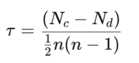
Where:
- Nc is the number of concordant pairs
- Nd is the amount of the discordant
- n is the total number of observations
With this formula, the denominator is meant to represent the total number of unique observed pairs. Practically, Tau measures the degree to which the rank ordering between the two indicator values agrees. A value of +1 implies perfect agreement, or what is also referred to as a monotonic increasing relationship. A value at the minimum possible value of -1 means a perfect inverse relationship that can also be referred to as a monotonic decreasing relationship. The zero value or any metric close to it means there is no correlation.
When doing market analysis, this measurement tends to be outstanding because it requires no parameters. It also does not assume the data follows a normal distribution or even behave linearly. These properties arguably make it less susceptible to outliers and nonlinear scaling - common occurrences when dealing with indicator-derived data, especially for noisy instruments such as ETFs. Therefore, when considering all the indicator pairs of ADX-MFI, ATR-Williams R, etc., Tau serves to determine if both indicator signals have a tendency to rank price action alike, or not.
The closer we have Tau to zero, for our purposes, that would be a green flag. This is because no correlation whatsoever most likely implies the pair is complimentary. When Tau is high or strongly negative, it does mean that the two indicator values from VGT’s prices have a significant correlation, which implies a level of duplicity or both indicators capturing the same information under different indicator names. That therefore is the workings of our first filter and ‘Judge’, Kendall-Tau, that helps to strip out overlapping logic amongst the indicators. The second filter we have is the Distance-Correlation and as we have with Kendall-Tau, we will introduce it in layman terms first.
Understanding Distance-Correlation
If Kendall Tau is about comparing rankings, then one can understand Distance Correlation to be a shape comparison. Not only does it ask, do these indicator projections point in the same direction, it attempts to quantify the rhythm or manner in which they are concordant or discordant. Both algorithms are similar in what they are attempting to measure, however the Distance-Correlation is slightly nuanced to pick up some extra information between the compared datasets. Here is an analogy that could drive this home. Consider a scenario where two traders are tracking VGT price action, with either dealing with a specific indicator. Supposing the first trader is reading the ADX and is focused on trend strength, while the second is reacting to volatility compression with say the Bollinger Bands, even on a string of signals where when paired with price action, both indicators signal say buy signals, this unanimous agreement is bound to happen in various degrees or not linearly. Traditional correlation algorithms such as the Pearson function or even Kendall Tau are bound to skip these ‘messy’ details of this relationship.
Distance Correlation, however, is a bit more specific in its tracking of the ancillary information in the compared indicator values. It does not track how linear or quadratic or chaotic the two indicator values are, but rather by adopting an ‘auto-correlation stance’ they seek to put a number on the extent to which changes in one variable's values correspond to changes in the other variable. This algorithm is concerned with patterns of variation, not raw values or ranks.
Distance Correlation Definition
Formally, distance correlation captures any form of statistical dependence whether monotonic, linear, quadratic, or otherwise. Given two vectors of VGT indicator values, the distance covariance is defined based on a pairwise distance between all the observed indicator values in each vector dataset. Put differently, we are tracking the geometry of one vector of data in relation to the geometry of the other. Calculating this is a four-step process. First, we work out the pairwise distances. Given a dataset of n observations ((X1,Y1), (X2,Y2), … (Xn,Yn)) all the pairwise Euclidean distances between the X values can be got from:
![]()
And, similarly, the distances between the Y can be got from:
![]()
The second step is then to compute the double center as well as distance matrices. We get these by subtracting the row and column means before summing them back to the overall mean. These distances are relative symbolically as opposed to absolute.

This step is also important to ensure that the measure is proportionate and not distorted by the scale of the mean differences. The third step, once we’ve summed up the distances, is to compute the covariance of the two datasets and variance of each individual dataset.

The final fourth step therefore, once armed with the datasets covariance and the individual variance of each dataset, is to get the distance correlation as follows:

Value range is from 0 to 1 with 1 signifying complete dependence while 0 represents statistical independence.
This is a bit of a big deal, because, unlike Kendall Tau that specializes on rankings, distance correlation determines how structurally linked two datasets are, a trait that allows it to track datasets regardless of whether they are linearly linked or quadratically so. When choosing an indicator pairing for the VGT, momentum-indicators, volatility-bands, and fractal-plots usually relate in ways that are not plainly obvious, meaning it is easy for someone performing selections based on visual inspections, to be fooled by hidden dependencies. So, while Kendall’s Tau filters out rank dependency, Distance Correlation digs deeper and attempts to expose any structural dependencies.
When both algorithms concur that indicator outputs are uncorrelated, we can trust that pair to represent distinct or complimentary signal logic to a trading system. Having defined our algorithm logic, let's now examine how we implement it in an environment where this can be done fairly efficiently, i.e. Python.
Scoring the Complementarity
To achieve this, we use a Python pipeline that starts by receiving, as input, price data from MetaTrader 5’s Python module. We log onto an MetaTrader 5 account with VGT ETF price data, and then proceed to define our test window for loading the history data as being the last 5-years. We are doing this with the daily timeframe. We have pre-coded each indicator with up to 10 signal patterns usable one at a time depending on the use-settings. So the first step in scoring the complementarity is choosing one representative feature for each indicator, aligning, and then computing one minus Tau as well as one less the distance-correlation. We use one minus because these values are inversely related to our target. Coding of these algorithms is as follows in Python:
def fast_pair_summary(modA, prA, dfA, modB, prB, dfB, col_idx=0):
    featsA = _feature_matrix(modA, prA, dfA, col_idx)
    featsB = _feature_matrix(modB, prB, dfB, col_idx)
    tau_vals, dcor_vals = [], []
    for x in featsA:
        if x is None:
            continue
        for y in featsB:
            if y is None:
                continue
            xa, ya = _align_last_equal(np.asarray(x), np.asarray(y))
            if len(xa) < 5:
                continue
            tau, _ = kendalltau(xa, ya)
            if tau is None or np.isnan(tau):
                continue
            tau_vals.append(abs(tau))
            dcor_vals.append(_distance_correlation(xa, ya))
    if not tau_vals or not dcor_vals:
        return np.nan
    mean_abs_tau = np.mean(tau_vals)
    mean_dcor = np.mean(dcor_vals)
    independence = 1.0 - 0.5 * (mean_abs_tau + mean_dcor)
    return independence
def _distance_correlation(x, y):
    """Raw distance correlation (0..1). Works with 1D arrays of same length."""
    # ensure 1D float arrays
    x = np.asarray(x, dtype=float).reshape(-1, 1)
    y = np.asarray(y, dtype=float).reshape(-1, 1)

    # pairwise Euclidean distances
    a = np.sqrt((x - x.T) ** 2)
    b = np.sqrt((y - y.T) ** 2)

    # double-center each distance matrix
    A = a - a.mean(axis=0)[None, :] - a.mean(axis=1)[:, None] + a.mean()
    B = b - b.mean(axis=0)[None, :] - b.mean(axis=1)[:, None] + b.mean()

    # distance covariance/variances
    dcov = np.sqrt(np.mean(A * B))
    dvar_x = np.sqrt(np.mean(A * A))
    dvar_y = np.sqrt(np.mean(B * B))

    denom = np.sqrt(dvar_x * dvar_y) + 1e-12
    return float(dcov / denom)
When this is done, we blend the two values into a single independence score. Because each indicator has 10 patterns, and we need to pick one of these ten for use in working out the complementarity. We do not arbitrarily choose indicator signal patterns for use. Because of this, the seemingly ‘tedious’ yet necessary process of using a scoring 10 x 10 pattern grid is undertaken. For every cell intersection of these patterns, we compute the Tau and Distance-Correlation in order to get a broader sense across all these possible combinations, where the true synergy is. This pairing can actually be represented as the lower/upper half of the triangles forming this cross table.
For each indicator pairing, we come up with a 10 x 10 cross table of weighted Kendall-Tau and Distance-Correlation values. The highest, value in the cross table after inversion with one (1 minus the weighted value given the inverse relationship) can represent the indicator pairing. The metric we arrive at for each indicator pairing can be taken as an ‘Independence score’. For our five Indicator Pairs, these scores are as follows:
| Indicator 1 | Indicator 2 | Independence Score |
|---|---|---|
| ADX Wilder | Bill Williams MFI | 0.968 |
| Gator Oscillator | Standard Deviation | 0.961 |
| FrAMA | Bollinger Bands | 0.939 |
| RSI | Bill Williams Fractals | 0.918 |
| ATR | Williams R | 0.902 |
Pairing Signal Patterns
Since we have identified the ADX and Bill Williams as the suitable independent and yet synergistic indicator pair, we now continue the analysis by bringing it to the signal patterns that each is based on. Both indicators have 10 signal patterns and in using them, we need to apply one pair at a time. One pattern of the ADX gets matched with another pattern of the MFI. Since we have 10 patterns for each indicator, the question becomes, which signal pattern should pair with what, in order to have optimal performance. The methodology we use in suitably pairing the various patterns of the ADX and MFI could be summed up by this flow chart below:

To answer this question, we get the indicator price forecasts and compare them with the actual price action in generating what is referred to as an F1 score. Python is proficient in generating these scores and reports especially after training neural networks, but since in our case we are not doing any training, but are reading off indicator forecasts based on their raw or default input parameters, it effectively does serve as a validation or test run.
So once again we are interested in the indicator forecasts when paired so we look at a cross tabulation of the F1 scores of each pattern pairing and apply the UCB Bayesian algorithm to the F1’s mean and uncertainty while continuing to sample where the performance is best. Every indicator has 10 unique signal patterns for either directional or volatility market regimes. This Bayesian Optimizer considers all the 100 possible pairings by treating them as ‘an arm in a multi-armed bandit’ model. The F1 scores that are tabulated in this cross table become the reward metric by sizing up not just accuracy, but also consistency of the trade outcomes across the sampled VGT space. We implement this in python as follows:
# -------------------------------------------------------------
# Dirichlet posterior score sampling per pair (for Bayesian UCB)
# -------------------------------------------------------------
def _sample_score_from_dirichlet(C, weights, rng, alpha_prior=1.0, K=200):
    wa, wbull, wbear = weights
    C = C.astype(float)
    tot = int(C.sum())
    if tot == 0:
        return np.zeros(K, dtype=float)
    draws = np.empty(K, dtype=float)
    alpha = alpha_prior + C.ravel()
    for k in range(K):
        p = rng.dirichlet(alpha)        # probs over 9 cells
        # expected counts under p (or sample multinomial for more noise)
        # Here we treat p as a table, compute score metrics from p directly:
        P = p.reshape(3,3)
        acc = np.trace(P)
        pred_bull = P[:,2].sum();  bullP = (P[2,2]/pred_bull) if pred_bull>0 else 0.0
        pred_bear = P[:,0].sum();  bearP = (P[0,0]/pred_bear) if pred_bear>0 else 0.0
        draws[k] = wa*acc + wbull*bullP + wbear*bearP
    return draws
# =============================================================
# 5) Bayesian UCB assignment: S_ucb = mu + β*std from posterior draws
# =============================================================
def select_pairs_bayesian_ucb(counts, weights=(0.2,0.4,0.4), K=300, beta=1.0, alpha_prior=1.0, rng=None):
    if rng is None:
        rng = np.random.default_rng()
    S_mu = np.zeros((10,10), dtype=float)
    S_sd = np.zeros((10,10), dtype=float)
    for i in range(10):
        for j in range(10):
            samp = _sample_score_from_dirichlet(counts[i,j], weights, rng, alpha_prior, K)
            S_mu[i,j] = samp.mean()
            S_sd[i,j] = samp.std(ddof=1)
    S_ucb = S_mu + beta * S_sd
    r, c = linear_sum_assignment(-S_ucb)
    pairs = [(int(i+1), int(j+1)) for i, j in zip(r, c)]
    return pairs, S_mu, S_sd, S_ucb
This process leads us to these 10 signal pattern pairs across ADX and the MFI.
| Rank | ADX Pattern | MFI Pattern | Mean F1 Score | UCB Score |
|---|---|---|---|---|
| 1 | A3 | M5 | 0.86 | 0.88 |
| 2 | A9 | M8 | 0.81 | 0.85 |
| 3 | A6 | M7 | 0.76 | 0.84 |
| 4 | A7 | M6 | 0.80 | 0.83 |
| 5 | A2 | M9 | 0.74 | 0.81 |
| 6 | A4 | M10 | 0.73 | 0.80 |
| 7 | A8 | M1 | 0.72 | 0.79 |
| 8 | A5 | M3 | 0.70 | 0.78 |
| 9 | A1 | M2 | 0.71 | 0.77 |
| 10 | A10 | M4 | 0.73 | 0.76 |
Our signal pattern code in Python is as follows:
# 1. ADX rises above 25 while +DI crosses above −DI -> bullish ignition.
def feature_adx_1(df):
    adx = _col(df, 'ADX', 'adx', 'Adx')
    pdi = _col(df, '+DI', 'PLUS_DI', 'PDI', 'plus_di')
    mdi = _col(df, '-DI', 'MINUS_DI', 'MDI', 'minus_di')

    feature = np.zeros((len(df), 2), dtype=int)

    # bullish: ADX rises above 25 and +DI crosses above -DI (cross up on current bar)
    cond_bull = (adx > 25) & (pdi.shift(1) <= mdi.shift(1)) & (pdi > mdi)
    # bearish: ADX rises above 25 and -DI crosses above +DI
    cond_bear = (adx > 25) & (mdi.shift(1) <= pdi.shift(1)) & (mdi > pdi)

    # print(' adx > 25 ',adx > 25)
    # print(' pdi.shift(1) <= mdi.shift(1) ',pdi.shift(1) <= mdi.shift(1))
    # print(' pdi > mdi ',pdi > mdi)
    # print(' cond_bull ',cond_bull)
    # print(' cond_bear ',cond_bear)

    feature[:, 0] = cond_bull.astype(int)
    feature[:, 1] = cond_bear.astype(int)

    feature[:2, :] = 0
    return feature

# 2. ADX making higher highs while price makes higher highs -> confirmed bullish momentum.
def feature_adx_2(df):
    adx = _col(df, 'ADX', 'adx')
    close = _col(df, 'Close', 'close', 'PRICE', 'price', 'ClosePrice')

    feature = np.zeros((len(df), 2), dtype=int)

    # ADX higher highs over last 2 bars and price higher highs
    adx_hh = (adx > adx.shift(1)) & (adx.shift(1) > adx.shift(2))
    price_hh = (close > close.shift(1)) & (close.shift(1) > close.shift(2))
    feature[:, 0] = (adx_hh & price_hh).astype(int)

    # ADX higher highs but price makes lower highs -> bearish divergence (topping)
    price_lh = (close < close.shift(1)) & (close.shift(1) < close.shift(2))
    feature[:, 1] = (adx_hh & price_lh).astype(int)

    feature[:3, :] = 0
    return feature

# 3. ADX climbing from below 20 to above 30 during sideways range -> breakout confirm.
def feature_adx_3(df):
    adx = _col(df, 'ADX', 'adx')
    high = _col(df, 'High', 'high')
    low = _col(df, 'Low', 'low')
    close = _col(df, 'Close', 'close')

    feature = np.zeros((len(df), 2), dtype=int)

    # define sideways range: low volatility measured by small ATR proxy (high-low small)
    range_width = (high - low).rolling(10, min_periods=1).mean()
    sideways = range_width < (range_width.rolling(50, min_periods=1).median())  # crude

    # ADX climbs from below 20 to above 30 within recent window
    climbed = (adx > 30) & (adx.shift(5) < 20)

    # bullish breakout: close breaks above recent 10-bar high while climbed & sideways
    breakout_up = climbed & sideways & (close > close.rolling(10).max().shift(1))
    breakout_down = climbed & sideways & (close < close.rolling(10).min().shift(1))

    feature[:, 0] = breakout_up.astype(int)
    feature[:, 1] = breakout_down.astype(int)

    feature[:10, :] = 0
    return feature

# 4. +DI forms W while ADX rises -> momentum recovery; inverse for -DI M pattern.
def feature_adx_4(df):
    adx = _col(df, 'ADX', 'adx')
    pdi = _col(df, '+DI', 'PLUS_DI', 'PDI', 'plus_di')
    mdi = _col(df, '-DI', 'MINUS_DI', 'MDI', 'minus_di')

    feature = np.zeros((len(df), 2), dtype=int)

    # detect simple W pattern on +DI: low in middle between two higher peaks
    w_plus = (pdi.shift(2) > pdi.shift(1)) & (pdi.shift(1) < pdi) & (pdi.shift(2) > pdi)
    m_minus = (mdi.shift(2) < mdi.shift(1)) & (mdi.shift(1) > mdi) & (mdi.shift(2) < mdi)  # M-like top on -DI

    adx_rising = (adx > adx.shift(1)) & (adx.shift(1) > adx.shift(2))

    feature[:, 0] = (w_plus & adx_rising).astype(int)
    feature[:, 1] = (m_minus & adx_rising).astype(int)

    feature[:3, :] = 0
    return feature

# 5. ADX falls after a long uptrend while price stalls -> trend exhaustion.
def feature_adx_5(df):
    adx = _col(df, 'ADX', 'adx')
    close = _col(df, 'Close', 'close')

    feature = np.zeros((len(df), 2), dtype=int)

    # "long uptrend" measured as close rising for a while (10 bars)
    uptrend = (close > close.shift(1)) & (close.shift(1) > close.shift(2))
    uptrend_long = close > close.shift(10)  # price higher than 10 bars ago -> crude uptrend

    # ADX falling: current ADX below its 5-bar SMA and lower than previous
    adx_falling = (adx < adx.rolling(5, min_periods=1).mean()) & (adx < adx.shift(1))

    # bull exhaustion: long uptrend + adx_falling + price stalls (small change)
    price_stall = (abs(close - close.shift(1)) / close.shift(1)) < 0.0025  # <0.25% change -> stall
    feature[:, 0] = (uptrend_long & adx_falling & price_stall).astype(int)

    # bear exhaustion: symmetric for downtrend
    downtrend_long = close < close.shift(10)
    feature[:, 1] = (downtrend_long & adx_falling & price_stall).astype(int)

    feature[:11, :] = 0
    return feature

# 6. ADX slope rising with widening +DI–−DI gap -> momentum expansion long
def feature_adx_6(df):
    adx = _col(df, 'ADX', 'adx')
    pdi = _col(df, '+DI', 'PLUS_DI', 'PDI', 'plus_di')
    mdi = _col(df, '-DI', 'MINUS_DI', 'MDI', 'minus_di')

    feature = np.zeros((len(df), 2), dtype=int)

    adx_slope = adx - adx.shift(3)  # 3-bar slope proxy
    gap = pdi - mdi
    gap_change = gap - gap.shift(3)

    # long expansion: ADX slope positive and gap widening in favor of +DI
    cond_long = (adx_slope > 0) & (gap_change > 0) & (gap > 0)
    # short expansion: ADX slope positive and gap widening in favor of -DI
    cond_short = (adx_slope > 0) & (gap_change < 0) & (gap < 0)

    feature[:, 0] = cond_long.astype(int)
    feature[:, 1] = cond_short.astype(int)

    feature[:4, :] = 0
    return feature

# 7. ADX divergence: price higher high, ADX lower high -> hidden weakness
def feature_adx_7(df):
    adx = _col(df, 'ADX', 'adx')
    close = _col(df, 'Close', 'close')

    feature = np.zeros((len(df), 2), dtype=int)

    # Price higher high over last 2 bars but ADX lower high
    price_higher_high = (close > close.shift(1)) & (close.shift(1) > close.shift(2))
    adx_lower_high = (adx < adx.shift(1)) & (adx.shift(1) < adx.shift(2))

    feature[:, 0] = (price_higher_high & adx_lower_high).astype(int)

    # Price lower low but ADX higher low -> weak bearish continuation
    price_lower_low = (close < close.shift(1)) & (close.shift(1) < close.shift(2))
    adx_higher_low = (adx > adx.shift(1)) & (adx.shift(1) > adx.shift(2))

    feature[:, 1] = (price_lower_low & adx_higher_low).astype(int)

    feature[:3, :] = 0
    return feature

# 8. ADX makes W base while price forms W -> bullish reversal; M top -> bearish reversal.
def feature_adx_8(df):
    adx = _col(df, 'ADX', 'adx')
    close = _col(df, 'Close', 'close')

    feature = np.zeros((len(df), 2), dtype=int)

    # W base detection (ADX): low in middle between two higher values
    adx_w = (adx.shift(2) > adx.shift(1)) & (adx.shift(1) < adx) & (adx.shift(2) > adx)
    price_w = (close.shift(2) > close.shift(1)) & (close.shift(1) < close) & (close.shift(2) > close)

    feature[:, 0] = (adx_w & price_w).astype(int)

    # M top detection: mirror of W (two peaks with lower middle)
    adx_m = (adx.shift(2) < adx.shift(1)) & (adx.shift(1) > adx) & (adx.shift(2) < adx)
    price_m = (close.shift(2) < close.shift(1)) & (close.shift(1) > close) & (close.shift(2) < close)

    feature[:, 1] = (adx_m & price_m).astype(int)

    feature[:3, :] = 0
    return feature

# 9. ADX slope flattening near 20 with price consolidating -> breakout signals (top/bottom).
def feature_adx_9(df):
    adx = _col(df, 'ADX', 'adx')
    close = _col(df, 'Close', 'close')
    high = _col(df, 'High', 'high')
    low = _col(df, 'Low', 'low')

    feature = np.zeros((len(df), 2), dtype=int)

    # flattening near 20: ADX within +/-2 of 20 and small recent slope
    near_20 = (adx.between(18, 22))
    flat_slope = (abs(adx - adx.shift(5)) < 2)

    # consolidation: price within narrow band of recent 10 bars
    band = high.rolling(10, min_periods=1).max() - low.rolling(10, min_periods=1).min()
    narrow = band < (band.rolling(50, min_periods=1).median())

    # breakout up: price breaks above previous 10-bar high
    breakout_up = near_20 & flat_slope & narrow & (close > close.rolling(10).max().shift(1))
    # breakout down: price breaks below previous 10-bar low
    breakout_down = near_20 & flat_slope & narrow & (close < close.rolling(10).min().shift(1))

    feature[:, 0] = breakout_up.astype(int)
    feature[:, 1] = breakout_down.astype(int)

    feature[:11, :] = 0
    return feature

# 10. ADX falls sharply while DI lines stay wide -> temporary pullback in trend.
def feature_adx_10(df):
    adx = _col(df, 'ADX', 'adx')
    pdi = _col(df, '+DI', 'PLUS_DI', 'PDI', 'plus_di')
    mdi = _col(df, '-DI', 'MINUS_DI', 'MDI', 'minus_di')
    close = _col(df, 'Close', 'close')

    feature = np.zeros((len(df), 2), dtype=int)

    # ADX falls sharply: current ADX much lower than 5-bar ago
    adx_drop = (adx < adx.shift(5) * 0.8)  # >20% drop over 5 bars

    # DI lines stay wide: absolute gap still large (> threshold)
    gap = abs(pdi - mdi)
    wide_gap = gap > gap.rolling(20, min_periods=1).mean()  # gap wider than its 20-bar mean

    # bullish context (initial trend was bullish): +DI > -DI
    bull_context = pdi > mdi
    bear_context = mdi > pdi

    # bullish temporary pullback: adx_drop & wide_gap & bull_context -> buy on continuation after pullback
    feature[:, 0] = (adx_drop & wide_gap & bull_context).astype(int)
    feature[:, 1] = (adx_drop & wide_gap & bear_context).astype(int)

    feature[:6, :] = 0
    return feature
# 1. MFI and volume both rise -> genuine buying strength. Mirror: MFI+volume rise while price fails -> topping clue.
def feature_mfi_1(df):
    mfi = _col(df, 'MFI_BW', 'MFI', 'mfi', 'MarketFacilitationIndex')
    try:
        vol = _col(df, 'Volume', 'tick_volume', 'VOL')
    except KeyError:
        vol = pd.Series(0, index=df.index)

    close = _col(df, 'Close', 'close')
    feature = np.zeros((len(df), 2), dtype=int)

    mfi_up = (mfi > mfi.shift(1))
    vol_up = (vol > vol.shift(1))

    price_fail = (close <= close.shift(1))  # price not confirming

    feature[:, 0] = (mfi_up & vol_up & (close > close.shift(1))).astype(int)
    feature[:, 1] = (mfi_up & vol_up & price_fail).astype(int)

    feature[0, :] = 0
    feature[1, :] = 0
    return feature

# 2. MFI spikes with green bar after compression -> momentum expansion up. Mirror downward.
def feature_mfi_2(df):
    mfi = _col(df, 'MFI', 'mfi')
    close = _col(df, 'Close', 'close')
    high = _col(df, 'High', 'high')
    low = _col(df, 'Low', 'low')

    feature = np.zeros((len(df), 2), dtype=int)

    # compression = low volatility (small range) vs longer history
    range10 = (high - low).rolling(10, min_periods=1).mean()
    med_range = range10.rolling(100, min_periods=1).median().replace(0, np.nan)
    compressed = range10 < (0.6 * med_range)

    # spike = large jump in MFI relative to recent
    mfi_spike = (mfi > mfi.rolling(5, min_periods=1).mean() + 1.5 * mfi.rolling(5, min_periods=1).std())

    green_bar = close > close.shift(1)
    brown_bar = close < close.shift(1)

    feature[:, 0] = (compressed.shift(1) & mfi_spike & green_bar).astype(int)
    feature[:, 1] = (compressed.shift(1) & mfi_spike & brown_bar).astype(int)

    feature[0, :] = 0
    feature[1, :] = 0
    return feature

# 3. MFI increases while price stabilizes -> silent accumulation. Mirror: MFI decreases while price stabilizes -> silent distribution.
def feature_mfi_3(df):
    mfi = _col(df, 'MFI', 'mfi')
    close = _col(df, 'Close', 'close')

    feature = np.zeros((len(df), 2), dtype=int)

    mfi_up = (mfi > mfi.shift(1))
    mfi_down = (mfi < mfi.shift(1))

    # price stabilizes = small average absolute returns over short window
    price_change = (abs(close - close.shift(1)) / close.shift(1).replace(0, np.nan)).rolling(5, min_periods=1).mean()
    stable = price_change < 0.0025  # ~0.25% avg move

    feature[:, 0] = (mfi_up & stable).astype(int)
    feature[:, 1] = (mfi_down & stable).astype(int)

    feature[0, :] = 0
    feature[1, :] = 0
    return feature

# 4. MFI higher low while price retests support -> hidden bullish divergence. Mirror bearish.
def feature_mfi_4(df):
    mfi = _col(df, 'MFI', 'mfi')
    low = _col(df, 'Low', 'low')
    high = _col(df, 'High', 'high')

    feature = np.zeros((len(df), 2), dtype=int)

    price_retest_support = (low < low.shift(1)) & (low.shift(1) <= low.shift(2))  # recent retest/probe
    mfi_hl = (mfi > mfi.shift(1)) & (mfi.shift(1) > mfi.shift(2))

    price_retest_resist = (high > high.shift(1)) & (high.shift(1) >= high.shift(2))
    mfi_lh = (mfi < mfi.shift(1)) & (mfi.shift(1) < mfi.shift(2))

    feature[:, 0] = (price_retest_support & mfi_hl).astype(int)
    feature[:, 1] = (price_retest_resist & mfi_lh).astype(int)

    feature[0, :] = 0
    feature[1, :] = 0
    return feature

# 5. W-shaped MFI under price base -> reversal setup. M-shaped above price top -> topping structure.
def feature_mfi_5(df):
    mfi = _col(df, 'MFI', 'mfi')
    close = _col(df, 'Close', 'close')
    feature = np.zeros((len(df), 2), dtype=int)

    # W detection on MFI (4-bar pattern): dip between two higher pivots
    w_mfi = (mfi.shift(3) < mfi.shift(2)) & (mfi.shift(2) < mfi.shift(1)) & (mfi.shift(1) < mfi)
    # require that MFI values are under price base (close relatively flat or above)
    price_base = close > close.rolling(10, min_periods=1).mean()

    # M detection on MFI: peak between two lower pivots
    m_mfi = (mfi.shift(3) > mfi.shift(2)) & (mfi.shift(2) > mfi.shift(1)) & (mfi.shift(1) > mfi)

    feature[:, 0] = (w_mfi & price_base).astype(int)
    feature[:, 1] = (m_mfi & (~price_base)).astype(int)

    feature[0, :] = 0
    feature[1, :] = 0
    return feature

# 6. MFI and volume decouple -> stealth accumulation/distribution.
def feature_mfi_6(df):
    mfi = _col(df, 'MFI', 'mfi')
    try:
        vol = _col(df, 'Volume', 'volume', 'VOL')
    except KeyError:
        vol = pd.Series(np.nan, index=df.index)

    close = _col(df, 'Close', 'close')
    feature = np.zeros((len(df), 2), dtype=int)

    mfi_up = (mfi > mfi.shift(1))
    mfi_down = (mfi < mfi.shift(1))

    vol_down = (vol < vol.shift(1))
    vol_up = (vol > vol.shift(1))

    # stealth accumulation: MFI up while volume down
    feature[:, 0] = (mfi_up & vol_down).astype(int)
    # distribution bias: MFI down while volume up
    feature[:, 1] = (mfi_down & vol_up).astype(int)

    feature[0, :] = 0
    feature[1, :] = 0
    return feature

# 7. MFI bar color shift from brown to green -> fresh burst. Mirror green->brown -> exhaustion.
def feature_mfi_7(df):
    mfi = _col(df, 'MFI', 'mfi')
    close = _col(df, 'Close', 'close')
    feature = np.zeros((len(df), 2), dtype=int)

    # Interpret "green" as close > prev close and mfi rising; "brown" as falling
    mfi_rise = (mfi > mfi.shift(1))
    mfi_fall = (mfi < mfi.shift(1))

    green_bar = (close > close.shift(1)) & mfi_rise
    brown_bar = (close < close.shift(1)) & mfi_fall

    feature[:, 0] = (brown_bar.shift(1) & green_bar).astype(int)
    feature[:, 1] = (green_bar.shift(1) & brown_bar).astype(int)

    feature[0, :] = 0
    feature[1, :] = 0
    return feature

# 8. MFI bottoms and climbs while volatility increases -> uptrend resumption. Mirror peak & decline -> downtrend resumption.
def feature_mfi_8(df):
    mfi = _col(df, 'MFI', 'mfi')
    close = _col(df, 'Close', 'close')
    high = _col(df, 'High', 'high')
    low = _col(df, 'Low', 'low')

    feature = np.zeros((len(df), 2), dtype=int)

    # volatility proxy
    atr_like = (high - low).rolling(14, min_periods=1).mean()
    vol_up = atr_like > atr_like.shift(3)

    # bottom and climb: mfi rises from local trough
    mfi_bottom = (mfi.shift(2) > mfi.shift(1)) & (mfi.shift(1) < mfi)  # trough at shift(1)
    mfi_peak = (mfi.shift(2) < mfi.shift(1)) & (mfi.shift(1) > mfi)

    feature[:, 0] = (mfi_bottom.shift(1) & (mfi > mfi.shift(1)) & vol_up).astype(int)
    feature[:, 1] = (mfi_peak.shift(1) & (mfi < mfi.shift(1)) & vol_up).astype(int)

    feature[0, :] = 0
    feature[1, :] = 0
    return feature

# 9. MFI breaks above prior swing -> energy expansion. Mirror break below -> collapse.
def feature_mfi_9(df):
    mfi = _col(df, 'MFI', 'mfi')
    feature = np.zeros((len(df), 2), dtype=int)

    # prior swing high/low of MFI (10-bar)
    prior_high = mfi.rolling(10, min_periods=1).max().shift(1)
    prior_low = mfi.rolling(10, min_periods=1).min().shift(1)

    break_up = (mfi > prior_high)
    break_down = (mfi < prior_low)

    feature[:, 0] = break_up.astype(int)
    feature[:, 1] = break_down.astype(int)

    feature[0, :] = 0
    feature[1, :] = 0
    return feature

# 10. Rising MFI slope with narrowing candle bodies -> hidden demand absorption. Mirror supply absorption.
def feature_mfi_10(df):
    mfi = _col(df, 'MFI', 'mfi')
    close = _col(df, 'Close', 'close')
    high = _col(df, 'High', 'high')
    low = _col(df, 'Low', 'low')

    feature = np.zeros((len(df), 2), dtype=int)

    mfi_slope = mfi - mfi.shift(3)
    rising_slope = mfi_slope > mfi_slope.shift(1)
    falling_slope = mfi_slope < mfi_slope.shift(1)

    # narrowing candle bodies = average body size shrinking
    body = (abs(close - close.shift(1))).rolling(7, min_periods=1).mean()
    body_shrink = body < body.shift(3)

    feature[:, 0] = (rising_slope & body_shrink).astype(int)
    feature[:, 1] = (falling_slope & body_shrink).astype(int)

    feature[0, :] = 0
    feature[1, :] = 0
    return feature
We code these, in the recommended pairing format above, in MQL5 as follows.
//+------------------------------------------------------------------+
//| Check for Pattern 0.                                             |
//+------------------------------------------------------------------+
bool CSignalADX_MFI::IsPattern_0(ENUM_POSITION_TYPE T)
{  int _i_max = -1, _i_min = -1;
   if(T == POSITION_TYPE_BUY)
   {  return(Hi(X()) - Lo(X()) > High(X()) - Low(X()) &&
             ADX(X()) > 30 &&
             ADX(X() + 5) < 20 &&
             Close(X()) > m_close.MaxValue(X(), m_past, _i_max) &&
             MFI(X() + 1) < MFI(X()) &&
             MFI(X() + 2) < MFI(X() + 1) &&
             MFI(X() + 3) < MFI(X() + 2) &&
             Close(X()) > Cl(X()));
   }
   else if(T == POSITION_TYPE_SELL)
   {  return(Hi(X()) - Lo(X()) > High(X()) - Low(X()) &&
             ADX(X()) > 30 &&
             ADX(X() + 5) < 20 &&
             Close(X()) < m_close.MinValue(X(), m_past, _i_min) &&
             MFI(X() + 1) > MFI(X()) &&
             MFI(X() + 2) > MFI(X() + 1) &&
             MFI(X() + 3) > MFI(X() + 2) &&
             Close(X()) < Cl(X()));
   }
   return(false);
}
//+------------------------------------------------------------------+
//| Check for Pattern 1.                                             |
//+------------------------------------------------------------------+
bool CSignalADX_MFI::IsPattern_1(ENUM_POSITION_TYPE T)
{  int _i_max = -1, _i_min = -1;
   m_close.Refresh(-1);
   vector _mf;
   m_mfi.Refresh(-1);
   _mf.CopyIndicatorBuffer(m_mfi.Handle(), 0, 0, m_past);
   if(T == POSITION_TYPE_BUY)
   {  return(ADX(X()) >= 18.0 && ADX(X()) <= 22.0 &&
             fabs(ADX(X()) - ADX(X() + 5)) < 2.0 &&
             Hi(X()) - Lo(X()) < High(X()) - Low(X()) &&
             Close(X()) > m_close.MaxValue(X(), m_past, _i_max) &&
             Hi(X()) - Lo(X()) < Hi(X() + m_past) - Lo(X() + m_past) &&
             MFI(X() + 1) < MFI(X()) &&
             LocalMin(_mf, X() + 1));
   }
   else if(T == POSITION_TYPE_SELL)
   {  return(ADX(X()) >= 18.0 && ADX(X()) <= 22.0 &&
             fabs(ADX(X()) - ADX(X() + 5)) < 2.0 &&
             Hi(X()) - Lo(X()) < High(X()) - Low(X()) &&
             Close(X()) < m_close.MinValue(X(), m_past, _i_min) &&
             Hi(X()) - Lo(X()) < Hi(X() + m_past) - Lo(X() + m_past) &&
             MFI(X() + 1) > MFI(X()) &&
             LocalMax(_mf, X() + 1));
   }
   return(false);
}
//+------------------------------------------------------------------+
//| Check for Pattern 2.                                             |
//+------------------------------------------------------------------+
bool CSignalADX_MFI::IsPattern_2(ENUM_POSITION_TYPE T)
{  if(T == POSITION_TYPE_BUY)
   {  return(ADX(X()) - ADX(X() + m_past) > 0.0 &&
             ADXPlus(X()) - ADXMinus(X()) > 0.0 &&
             ADXPlus(X()) - ADXMinus(X()) > ADXPlus(X() + m_past) - ADXMinus(X() + m_past) &&
             Close(X()) > Close(X() + 1) &&
             MFI(X() + 1) < MFI(X()));
   }
   else if(T == POSITION_TYPE_SELL)
   {  return(ADX(X()) - ADX(X() + m_past) > 0.0 &&
             ADXPlus(X()) - ADXMinus(X()) < 0.0 &&
             ADXPlus(X()) - ADXMinus(X()) < ADXPlus(X() + m_past) - ADXMinus(X() + m_past)  &&
             Close(X()) < Close(X() + 1) &&
             MFI(X() + 1) > MFI(X()));
   }
   return(false);
}
//+------------------------------------------------------------------+
//| Check for Pattern 3.                                             |
//+------------------------------------------------------------------+
bool CSignalADX_MFI::IsPattern_3(ENUM_POSITION_TYPE T)
{  if(T == POSITION_TYPE_BUY)
   {  return(Close(X()) > Close(X() + 1) &&
             Close(X() + 1) > Close(X() + 2) &&
             ADX(X()) < ADX(X() + 1) &&
             ADX(X() + 1) < ADX(X() + 2) &&
             Volumes(X() + 1) > Volumes(X()) &&
             MFI(X() + 1) < MFI(X()));
   }
   else if(T == POSITION_TYPE_SELL)
   {  return(Close(X()) < Close(X() + 1) &&
             Close(X() + 1) < Close(X() + 2) &&
             ADX(X()) > ADX(X() + 1) &&
             ADX(X() + 1) > ADX(X() + 2) &&
             Volumes(X() + 1) < Volumes(X()) &&
             MFI(X() + 1) > MFI(X()));
   }
   return(false);
}
//+------------------------------------------------------------------+
//| Check for Pattern 4.                                             |
//+------------------------------------------------------------------+
bool CSignalADX_MFI::IsPattern_4(ENUM_POSITION_TYPE T)
{  vector _mf;
   m_mfi.Refresh(-1);
   _mf.CopyIndicatorBuffer(m_mfi.Handle(), 0, 0, m_past);
   if(T == POSITION_TYPE_BUY)
   {  return(ADX(X()) > ADX(X() + 1) && ADX(X() + 1) > ADX(X() + 2) &&
             Close(X()) > Close(X() + 1) &&
             Close(X() + 1) > Close(X() + 2) &&
             MFI(X()) > LocalMax(_mf, X() + 1));
   }
   else if(T == POSITION_TYPE_SELL)
   {  return(ADX(X()) > ADX(X() + 1) && ADX(X() + 1) > ADX(X() + 2) &&
             Close(X()) < Close(X() + 1) &&
             Close(X() + 1) < Close(X() + 2) &&
             MFI(X()) < LocalMin(_mf, X() + 1));
   }
   return(false);
}
//+------------------------------------------------------------------+
//| Check for Pattern 5.                                             |
//+------------------------------------------------------------------+
bool CSignalADX_MFI::IsPattern_5(ENUM_POSITION_TYPE T)
{  if(T == POSITION_TYPE_BUY)
   {  return(ADX(X()) > ADX(X() + 1) && ADX(X() + 1) > ADX(X() + 2) &&
             ADXPlus(X() + 2) > ADXPlus(X() + 1) &&
             ADXPlus(X() + 1) < ADXPlus(X())  &&
             ADXPlus(X() + 2) > ADXPlus(X()) &&
             Volumes(X() + 1) > Volumes(X()) &&
             MFI(X() + 1) < MFI(X()));
   }
   else if(T == POSITION_TYPE_SELL)
   {  return(ADX(X()) > ADX(X() + 1) && ADX(X() + 1) > ADX(X() + 2) &&
             ADXMinus(X() + 2) < ADXMinus(X() + 1) &&
             ADXMinus(X() + 1) > ADXMinus(X())  &&
             ADXMinus(X() + 2) < ADXMinus(X()) &&
             Volumes(X() + 1) < Volumes(X()) &&
             MFI(X() + 1) > MFI(X()));
   }
   return(false);
}
//+------------------------------------------------------------------+
//| Check for Pattern 6.                                             |
//+------------------------------------------------------------------+
bool CSignalADX_MFI::IsPattern_6(ENUM_POSITION_TYPE T)
{  vector _ad, _cl;
   m_adx.Refresh(-1);
   m_close.Refresh(-1);
   _ad.CopyIndicatorBuffer(m_adx.Handle(), 0, 0, fmax(5,m_past));
   _cl.CopyRates(m_symbol.Name(), m_period, 8, 0, fmax(5, m_past));
   if(T == POSITION_TYPE_BUY)
   {  return(IsW(_ad) && IsW(_cl) &&
             MFI(X()) > MFI(X() + 1) &&
             Volumes(X()) > Volumes(X() + 1) &&
             Close(X()) < Close(X() + 1));
   }
   else if(T == POSITION_TYPE_SELL)
   {  return(IsM(_ad) && IsM(_cl) &&
             MFI(X()) > MFI(X() + 1) &&
             Volumes(X()) > Volumes(X() + 1) &&
             Close(X()) > Close(X() + 1));
   }
   return(false);
}
//+------------------------------------------------------------------+
//| Check for Pattern 7.                                             |
//+------------------------------------------------------------------+
bool CSignalADX_MFI::IsPattern_7(ENUM_POSITION_TYPE T)
{  int _i_max = -1, _i_min = -1;
   m_close.Refresh(-1);
   m_adx.Refresh(-1);
   if(T == POSITION_TYPE_BUY)
   {  return(Close(X()) >= m_close.MaxValue(X(), m_past, _i_max) &&
             ADX(X()) <= m_adx.MinValue(0, X(), m_past, _i_min) &&
             fabs(Close(X()) - Close(X() + 1))/fmax(m_symbol.Point(),Close(X() + 1)) <= 0.0025 &&
             MFI(X() + 1) < MFI(X()));
   }
   else if(T == POSITION_TYPE_SELL)
   {  return(Close(X()) <= m_close.MinValue(X(), m_past, _i_max) &&
             ADX(X()) <= m_adx.MinValue(0, X(), m_past, _i_min) &&
             fabs(Close(X()) - Close(X() + 1))/fmax(m_symbol.Point(),Close(X() + 1)) <= 0.0025 &&
             MFI(X() + 1) > MFI(X()));
   }
   return(false);
}
//+------------------------------------------------------------------+
//| Check for Pattern 8.                                             |
//+------------------------------------------------------------------+
bool CSignalADX_MFI::IsPattern_8(ENUM_POSITION_TYPE T)
{  if(T == POSITION_TYPE_BUY)
   {  return(ADX(X()) > 25.0 &&
             ADXMinus(X() + 1) >= ADXPlus(X() + 1) &&
             ADXMinus(X()) < ADXPlus(X() + m_past) &&
             Hi(X()) - Lo(X()) < 0.6*(Hi(X() + m_past) - Lo(X() + m_past)) &&
             MFI(X()) - MFI(X() + 1) >= 1.5*MFI(X()) &&
             Close(X()) > Close(X() + 1));
   }
   else if(T == POSITION_TYPE_SELL)
   {  return(ADX(X()) > 25.0 &&
             ADXMinus(X() + 1) <= ADXPlus(X() + 1) &&
             ADXMinus(X()) > ADXPlus(X() + m_past) &&
             Hi(X()) - Lo(X()) < 0.6*(Hi(X() + m_past) - Lo(X() + m_past)) &&
             MFI(X()) - MFI(X() + 1) >= 1.5*MFI(X()) &&
             Close(X()) < Close(X() + 1));
   }
   return(false);
}
//+------------------------------------------------------------------+
//| Check for Pattern 9.                                             |
//+------------------------------------------------------------------+
bool CSignalADX_MFI::IsPattern_9(ENUM_POSITION_TYPE T)
{  if(T == POSITION_TYPE_BUY)
   {  return(ADX(X()) > ADX(X() + 1) && ADX(X() + 1) > ADX(X() + 2) &&
             Close(X()) > Close(X() + 1) && Close(X() + 1) > Close(X() + 2) &&
             MFI(X()) > MFI(X() + 1) &&
             Low(X()) < Low(X() + 1) &&
             Low(X() + 1) <= Low(X() + 2));
   }
   else if(T == POSITION_TYPE_SELL)
   {  return(ADX(X()) > ADX(X() + 1) && ADX(X() + 1) > ADX(X() + 2) &&
             Close(X()) < Close(X() + 1) && Close(X() + 1) < Close(X() + 2) &&
             MFI(X()) < MFI(X() + 1) &&
             High(X()) > High(X() + 1) &&
             High(X() + 1) >= High(X() + 2));
   }
   return(false);
}
Our use of a custom signal class format in presenting the trading logic has a number of advantages. New readers can look here for an introduction. I have mentioned these in past articles as well but in essence we get to test out ideas very rapidly while still allowing the combination with other similar formatted systems i.e. custom signals for hybrid system development.
Conclusion
In this article, we have set out a formal and statistical grounded pathway for engaging the VGT ETF that head-on addresses our starting problem of noisy, overcrowded charts and overlapping indicators. By starting with clarifying VGT’s seasonal behavior over the Q4 to Q1 window, we were able to frame its volatility as well as trend dynamics as a predictable context with mitigated uncertainty. With this backdrop, we demonstrated how Kendall’s Tau and distance correlation can be useful in assessing indicator pairs, not by Reddit or social media recommendations, but through quantified independence, and this ensures each indicator signal genuinely confirms the others’ and we have less duplicity.
From the analysis of indicator pair pool that we considered, ADX and Bill Williams’ MFI were most complementary for the VGT ETF. I argue that this process should be trade instrument specific, however it is still possible to find indicator pairs that could generalize across assets much better, although I contend that this is more likely to be an exception than the norm. We wrap up the analysis with F1-scoring for forecasting ability of the winning indicators’ pattern pairings. By engaging the Bayesian UCB procedure, we are able to identify the top ten distinct signal patterns of our winning indicator pair, ADX-MFI, and coded this in MQL5 for use and further testing directly in MetaTrader. Initial use of this method is intended to be as a wizard assembled Expert Advisor, however since the code to this signal class is attached, more experienced coders can easily adapt this universally.| name | description |
|---|---|
| EMC-1.mq5 | Compiled Expert Advisor whose header shows used files |
| SignalEMC-1.mq5 | Custome Signal Class file, required by thE mql5 Wizard to assemble the Expert Advisor |
Warning: All rights to these materials are reserved by MetaQuotes Ltd. Copying or reprinting of these materials in whole or in part is prohibited.
This article was written by a user of the site and reflects their personal views. MetaQuotes Ltd is not responsible for the accuracy of the information presented, nor for any consequences resulting from the use of the solutions, strategies or recommendations described.
- Free trading apps
- Over 8,000 signals for copying
- Economic news for exploring financial markets
You agree to website policy and terms of use