将MQL5与数据处理软件包集成(第 5 部分):自适应学习与灵活性
 66
 0

引言
许多算法交易者面临的问题在于传统交易系统的僵化性和缺乏适应性。如前一篇文章所述,大多数基于规则的 EA 都采用静态条件和阈值的硬编码方式,这往往无法实时适应不断变化的市场动态、波动性变化或未见模式。因此,这些系统在特定市场状态下表现良好,但当市场行为发生变化时,其性能会恶化,从而导致错失机会、频繁发出错误信号或持续较长时间的资金回撤。
自适应学习和灵活性模式为这一问题提供了极具吸引力的解决方案。通过使用 Python 构建一个能够不断从历史 XAUUSD 价格行为中学习的强化学习模型,我们使系统能够根据不断变化的市场条件调整其策略。Python 库(如 PyTorch、Gym、Pandas 等)的灵活性支持高级数据预处理、环境模拟和模型优化。模型训练完成后,即可导出到 ONNX,从而能够在 MQL5 环境中部署。
获取历史数据
from datetime import datetime
import MetaTrader5 as mt5
import pandas as pd
import pytz

# Display data on the MetaTrader 5 package
print("MetaTrader5 package author: ", mt5.__author__)
print("MetaTrader5 package version: ", mt5.__version__)

# Configure pandas display options
pd.set_option('display.max_columns', 500)
pd.set_option('display.width', 1500)

# Establish connection to MetaTrader 5 terminal
if not mt5.initialize():
    print("initialize() failed, error code =", mt5.last_error())
    quit()

# Set time zone to UTC
timezone = pytz.timezone("Etc/UTC")
# Create 'datetime' objects in UTC time zone to avoid the implementation of a local time zone offset
utc_from = datetime(2025, 05, 15, tzinfo=timezone.utc)
utc_to = datetime.(2025, 07,08, tzinfo=timezone.utc)

# Get bars from XAU H1 (hourly timeframe) within the specified interval
rates = mt5.copy_rates_range("XAUUSD", mt5.TIMEFRAME_H1, utc_from, utc_to)

# Shut down connection to the MetaTrader 5 terminal
mt5.shutdown()

# Check if data was retrieved
if rates is None or len(rates) == 0:
    print("No data retrieved. Please check the symbol or date range.")
else:
    # Display each element of obtained data in a new line (for the first 10 entries)
    print("Display obtained data 'as is'")
    for rate in rates[:10]:
        print(rate)

    # Create DataFrame out of the obtained data
    rates_frame = pd.DataFrame(rates)
    # Convert time in seconds into the 'datetime' format
    rates_frame['time'] = pd.to_datetime(rates_frame['time'], unit='s')

    # Save the data to a CSV file
    filename = "XAU_H1.csv"
    rates_frame.to_csv(filename, index=False)
    print(f"\nData saved to file: {filename}")
为了检索历史数据,我们首先使用 mt5.initialize() 函数初始化与 MetaTrader 5 终端的连接,该函数实现了 Python 与 MetaTrader 5 平台之间的通信。随后,我们通过设置起始日期和结束日期来界定数据提取的具体日期范围。这些日期以 UTC 格式的 datetime 对象进行处理,以确保跨时区的一致性。在本例中,脚本被配置为使用 mt5.copy_rates_range() 函数请求 XAUUSD 交易品种的历史每小时数据,涵盖 2025 年 5 月 15 日至 2025 年 7 月 8 日期间。
filename = "XAUUSD_H1.csv"
rates_frame.to_csv(filename, index=False)
print(f"\nData saved to file: {filename}")
您可能已经知道,我的操作系统是Linux。如果您的操作系统是 Windows,您可以使用以下 Python 脚本轻松获取历史数据:
from datetime import datetime
import MetaTrader5 as mt5
import pandas as pd
import pytz

# Display data on the MetaTrader 5 package
print("MetaTrader5 package author: ", mt5.__author__)
print("MetaTrader5 package version: ", mt5.__version__)

# Configure pandas display options
pd.set_option('display.max_columns', 500)
pd.set_option('display.width', 1500)

# Establish connection to MetaTrader 5 terminal
if not mt5.initialize():
    print("initialize() failed, error code =", mt5.last_error())
    quit()

# Set time zone to UTC
timezone = pytz.timezone("Etc/UTC")
# Create 'datetime' objects in UTC time zone to avoid the implementation of a local time zone offset
utc_from = datetime(2025, 05, 15, tzinfo=timezone.utc)
utc_to = datetime(2025, 07, 08, tzinfo=timezome.utc)

# Get bars from XAUUSD H1 (hourly timeframe) within the specified interval
rates = mt5.copy_rates_range("XAUUSD", mt5.TIMEFRAME_H1, utc_from, utc_to)

# Shut down connection to the MetaTrader 5 terminal
mt5.shutdown()

# Check if data was retrieved
if rates is None or len(rates) == 0:
    print("No data retrieved. Please check the symbol or date range.")
else:
    # Display each element of obtained data in a new line (for the first 10 entries)
    print("Display obtained data 'as is'")
    for rate in rates[:10]:
        print(rate)

    # Create DataFrame out of the obtained data
    rates_frame = pd.DataFrame(rates)
    # Convert time in seconds into the 'datetime' format
    rates_frame['time'] = pd.to_datetime(rates_frame['time'], unit='s')

    # Display data directly
    print("\nDisplay dataframe with data")
    print(rates_frame.head(10)
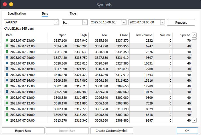
如果您无法通过编程方式检索历史数据,则可以直接从 MetaTrader 5 平台手动下载。首先启动平台,然后转到顶部菜单,导航至“工具”>“选项”,即可进入图表设置。在此,您需要指定图表上要显示的 K 线数量。建议选择“无限”选项,尤其是因为我们将处理日期范围,并且无法精确预测给定时间范围将包含多少根 K 线。
接下来,要下载实际数据,请在菜单栏中选择“查看”>“交易品种”,这将打开“规格”选项卡下的“交易品种”窗口。然后,根据您需要的数据类型,选择“柱”或“报价”选项卡。输入您希望获取的历史数据的开始日期和结束日期,然后单击“请求”按钮。数据检索完成后,您可以将其导出并以 .csv 格式保存,以便日后使用。
开始实现
import pandas as pd

# Load the uploaded BTC 1H CSV file
file_path = '/home/int_j/Documents/Art Draft/Data Science/Adaptive Learning/XAUUSD_H1.csv'
xau_data = pd.read_csv(file_path)

# Display basic information about the dataset
xau_data_info = xau_data.info()
xau_data_head = xau_data.head()

xau_data_info, xau_data_head
我们首先通过检查数据集来了解其结构。这包括使用 info() 函数检查数据类型、维度和完整性。此外,我们使用 head() 函数预览前几行,以了解数据集的内容和布局。这一步是探索性数据分析的标准部分,有助于确认数据是否已正确导入,并提供其格式的初步概览。
# Reload the data with tab-separated values
xau_data = pd.read_csv(file_path, delimiter='\t')

# Display basic information and the first few rows after parsing
xau_data_info = xau_data.info()
xau_data_head = xau_data.head()

xau_data_info, xau_data_head
此代码块首先从指定文件路径重新加载 XAUUSD 历史数据,使用制表符(\t)作为分隔符,而不是默认的逗号。处理 TSV(制表符分隔值)文件时,确保数据正确解析非常重要。将数据加载到 xau_data DataFrame 后,它使用 info() 函数打印出关于数据集的基本信息,如列类型、非空计数和内存使用情况,并使用 head() 函数显示前几行以进行快速预览。
import pandas as pd
import numpy as np
import ta
from sklearn.preprocessing import StandardScaler

# Split the single column into proper columns
if len(xau_data.columns) == 1:
    # Extract column headers from the first row
    headers = xau_data.columns[0].split('\t')

    # Split data into separate columns
    xau_data = xau_data[xau_data.columns[0]].str.split('\t', expand=True)
    xau_data.columns = headers

# Convert columns to proper data types
numeric_cols = ['<OPEN>', '<HIGH>', '<LOW>', '<CLOSE>', '<TICKVOL>', '<VOL>', '<SPREAD>']
xau_data[numeric_cols] = xau_data[numeric_cols].apply(pd.to_numeric, errors='coerce')

# Clean and create features
xau_data = xau_data.dropna()
xau_data['return'] = xau_data['<CLOSE>'].pct_change()

# Add technical indicators
xau_data['rsi'] = ta.momentum.RSIIndicator(xau_data['<CLOSE>'], window=14).rsi()
xau_data['macd'] = ta.trend.MACD(xau_data['<CLOSE>']).macd_diff()
xau_data['sma_20'] = ta.trend.SMAIndicator(xau_data['<CLOSE>'], window=20).sma_indicator()
xau_data['sma_50'] = ta.trend.SMAIndicator(xau_data['<CLOSE>'], window=50).sma_indicator()
xau_data = xau_data.dropna()

# Normalize features
scaler = StandardScaler()
features = ['rsi', 'macd', 'sma_20', 'sma_50', 'return']
xau_data[features] = scaler.fit_transform(xau_data[features])
在此代码块中,该过程首先从清理和格式化历史 XAUUSD 数据集开始。如果数据错误地加载为单列(这在制表符分隔的文件中可能发生),则脚本会使用制表符来拆分该列,以提取正确的标题和值。之后,它会明确地将开盘价、最高价、最低价、收盘价、交易量和点差等关键列转换为数值数据类型,并在转换过程中使用 errors='coerce' 来处理任何错误。然后,脚本会删除所有由此产生的缺失值,并添加一个新列用于计算每日收益率,即收盘价的百分比变化。
下一节将使用 TA(技术分析)库,通过技术指标来丰富数据集。RSI(相对强弱指数)、MACD(移动平均收敛/发散指标)和简单移动平均线(20周期和50周期)等指标均以收盘价为基础计算。这些特征常用于算法交易中,以帮助模型识别趋势和动量。最后,使用 scikit-learn 中的 StandardScaler 对所有选定的特征列进行标准化,以确保它们的均值为零,方差为 1,这是在将数据输入机器学习或强化学习模型进行训练之前必不可少的步骤。
import gym
from gym import spaces

class TradingEnv(gym.Env):
    def __init__(self, df, window_size=30, initial_balance=10000):
        super(TradingEnv, self).__init__()
        self.df = df.reset_index(drop=True)
        self.window_size = window_size
        self.initial_balance = initial_balance
        self.action_space = spaces.Discrete(3)  # 0: hold, 1: buy, 2: sell

        # Use correct shape (window_size, number of features)
        self.observation_space = spaces.Box(
            low=-np.inf, high=np.inf,
            shape=(self.window_size, len(features)), dtype=np.float32
        )

    def reset(self):
        self.current_step = self.window_size
        self.balance = self.initial_balance
        self.position = 0  # 1 = long, -1 = short, 0 = neutral
        self.entry_price = 0
        self.trades = []
        return self._next_observation()

    def _next_observation(self):
        # Use iloc to prevent overshooting shape
        obs = self.df.iloc[self.current_step - self.window_size : self.current_step]
        obs = obs[features].values
        return obs

    def step(self, action):
        current_price = self.df.loc[self.current_step, '<CLOSE>']
        reward = 0

        if action == 1 and self.position == 0:  # Buy
            self.position = 1
            self.entry_price = current_price
        elif action == 2 and self.position == 0:  # Sell
            self.position = -1
            self.entry_price = current_price
        elif action == 0 and self.position != 0:  # Close position
            if self.position == 1:
                reward = current_price - self.entry_price
            elif self.position == -1:
                reward = self.entry_price - current_price
            self.position = 0

        self.current_step += 1
        done = self.current_step >= len(self.df) - 1
        obs = self._next_observation()
        return obs, reward, done, {}
从上面的代码中,我们定义了一个名为 TradingEnv 的自定义 OpenAI Gym 环境,旨在利用历史金融数据集(在我们的例子中是 XAUUSD)训练强化学习代理进行交易决策。该环境通过允许三种离散动作来模拟交易:持有(0)、买入(1)或卖出(2)。它以过去观察数据的固定窗口(window_size)进行初始化,并使用数据中的特征来模拟交易行为。观察空间是一个历史特征值(例如,RSI、MACD)的窗口,环境会跟踪余额、持仓状态和入场价格等关键要素。
reset() 函数通过重置步数计数器、余额、持仓状态和任何未结交易来为新回合准备环境。step() 函数实现每个智能体动作的逻辑。如果智能体在没有持仓时买入或卖出,则开立一笔交易。如果智能体在已交易状态下选择持有,则平仓并计算盈亏作为奖励。回合通过数据集逐步进行,直至结束(done=True)。返回的观察值是历史特征的切片,智能体使用这些切片来做出未来决策。
import torch.nn as nn
import torch.nn.functional as F

class DuelingDQN(nn.Module):
    def __init__(self, state_shape, action_dim):
        super(DuelingDQN, self).__init__()
        # Calculate flattened dimension
        flattened_dim = np.prod(state_shape)

        # Network layers
        self.fc1 = nn.Linear(flattened_dim, 128)

        # Value stream
        self.value_stream = nn.Sequential(
            nn.Linear(128, 128),
            nn.ReLU(),
            nn.Linear(128, 1)
        )

        # Advantage stream
        self.advantage_stream = nn.Sequential(
            nn.Linear(128, 128),
            nn.ReLU(),
            nn.Linear(128, action_dim)
        )

    def forward(self, state):
        # Flatten state while keeping batch dimension
        x = state.view(state.size(0), -1)
        x = F.relu(self.fc1(x))
        value = self.value_stream(x)
        advantages = self.advantage_stream(x)
        return value + (advantages - advantages.mean(dim=1, keepdim=True))
现在,我们使用PyTorch定义了一个对偶深度 Q 网络(Dueling DQN),它是标准 DQN 架构的一种变体,将状态值函数的估计和优势函数的估计分开。DuelingDQN 类继承自 nn.Module,并接受输入状态的形状和可能动作的数量(action_dim)作为参数。它首先将输入状态展平,并通过一个共享的全连接层(fc1)。然后,输出被分为两路:一路用于估计状态值,另一路用于估计每个动作的优势。
在 forward() 方法中,两个数据流使用以下公式重新组合:

这确保了模型能够学会区分状态的内在价值(V(s))和采取每个可能动作的相对收益(A(s, a)),从而提高了基于价值的强化学习任务(如交易)的稳定性和性能。
# Training loop parameters
env = TradingEnv(xau_data)

# Use positional arguments instead of keyword arguments
model = DuelingDQN(150, 3)  # input_dim=150 (flattened state), action_dim=3
target_model = DuelingDQN(150, 3)  # Same dimensions
target_model.load_state_dict(model.state_dict())
输出:
<All keys matched successfully>
在这里,我们初始化对偶深度 Q 网络(Dueling DQN)智能体的训练环境和模型。TradingEnv 环境是使用预先准备好的 xau_data 创建的,它为强化学习提供市场特征。创建了 DuelingDQN 模型的两个实例:model(在线网络)和 target_model(目标网络),两者的扁平化输入维度均为 150,动作空间为 3(买入、卖出、持有)。target_model 是通过复制模型权重来初始化的,这是 DQN 训练中的标准做法,通过在时间差分更新期间使用更新缓慢的目标网络来稳定学习。
class ReplayBuffer:
    def __init__(self, capacity=10000):
        self.buffer = deque(maxlen=capacity)

    def push(self, state, action, reward, next_state, done):
        self.buffer.append((state, action, reward, next_state, done))

    def sample(self, batch_size):
        batch = random.sample(self.buffer, batch_size)
        state, action, reward, next_state, done = map(np.array, zip(*batch))
        return (
            torch.tensor(state, dtype=torch.float32),          # Shape: [batch, state_dim]
            torch.tensor(action, dtype=torch.int64),           # Should be integer (for indexing)
            torch.tensor(reward, dtype=torch.float32),
            torch.tensor(next_state, dtype=torch.float32),
            torch.tensor(done, dtype=torch.float32)
        )

    def __len__(self):
        return len(self.buffer)
ReplayBuffer 类实现了一个用于强化学习的内存缓冲区,用于存储和采样训练经验。它使用一个具有固定最大容量(默认值:10,000) 的双端队列来高效管理包含(state, action, reward, next_state, done)的元组的存储。push() 方法将新的经验添加到缓冲区中,当容量超过时会自动丢弃最旧的经验。
sample() 方法会随机选择一批经验,并将其转换为适用于模型训练的 PyTorch 张量,同时确保每个元素的数据类型都正确(例如,动作使用 int64 类型,状态和奖励使用 float32 类型)。此缓冲区支持稳定且不相关的学习,允许智能体从过去多样化的交互中学习,而不仅仅是连续的步骤。
env = TradingEnv(xau_data)
obs_shape = env.observation_space.shape
n_actions = env.action_space.n

# Calculate flattened dimension
flattened_dim = np.prod(obs_shape)  # 30*5 = 150

model = DuelingDQN(flattened_dim, n_actions)
target_model = DuelingDQN(flattened_dim, n_actions)
target_model.load_state_dict(model.state_dict())

optimizer = optim.Adam(model.parameters(), lr=0.0005)
buffer = ReplayBuffer()
gamma = 0.99
epsilon = 1.0
batch_size = 64
target_update_interval = 10

all_rewards = []
all_actions = []  # We'll collect actions for the entire dataset

# Training loop
for episode in range(200):
    state = env.reset()
    total_reward = 0
    done = False
    episode_actions = []  # Store actions for this episode

    while not done:
        if random.random() < epsilon:
            action = env.action_space.sample()
        else:
            with torch.no_grad():
                # Flatten state and pass to model
                state_tensor = torch.tensor(state, dtype=torch.float32).flatten().unsqueeze(0)
                q_values = model(state_tensor)
                action = q_values.argmax().item()

        next_state, reward, done, _ = env.step(action)
        buffer.push(state, action, reward, next_state, done)
        state = next_state
        total_reward += reward
        episode_actions.append(action)  # Record action

        if len(buffer) >= batch_size:
            s, a, r, s2, d = buffer.sample(batch_size)

            q_val = model(s).gather(1, a.unsqueeze(1)).squeeze()
            next_q_val = target_model(s2).max(1)[0]
            target = r + (1 - d) * gamma * next_q_val

            loss = nn.MSELoss()(q_val, target)
            optimizer.zero_grad()
            loss.backward()
            optimizer.step()

    epsilon = max(0.01, epsilon * 0.995)
    if episode % target_update_interval == 0:
        target_model.load_state_dict(model.state_dict())
        print(f"Episode {episode}, Reward: {total_reward}")

    # After episode completes
    all_rewards.append(total_reward)
    all_actions.extend(episode_actions)  # Add episode actions to master list
输出:
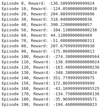
此训练循环使用对偶深度 Q 网络(对偶 DQN)为交易设置了一个强化学习环境。首先,使用历史 XAUUSD 数据初始化环境,并从观测空间和动作空间中推导出关键参数。创建了一个对偶 DQN 模型和一个目标模型,两者的输入形状均为150(表示 30 个时间步长 × 5 个特征)。设置了优化器(Adam)和经验回放缓冲区,以及折扣因子(gamma)、探索率(epsilon)、批量大小和目标网络更新频率等超参数。
在每个回合中,环境会被重置,智能体通过使用 ε-贪婪策略选择动作来逐步与环境交互。如果随机数小于 epsilon,则选择随机动作;否则,模型会选择预测 Q 值最高的动作。执行动作后,智能体会从环境中接收反馈,这些反馈会被存储在经验回放缓冲区中。当缓冲区拥有足够的数据后,就会从中采样一批经验来训练模型。计算 Q 值和目标值,并对均方误差损失进行反向传播以更新模型参数。
为了稳定训练,目标模型会定期更新以匹配当前模型的权重。随着时间的推移,ε 值会逐渐衰减以减少探索,从而使智能体能够更加自信地利用所学知识。整个训练过程中,会记录每回合的总奖励和动作,以进行性能评估。通过在 200 个回合中平衡探索和利用,这一循环有助于智能体学习最优的交易策略。
import matplotlib.pyplot as plt

# Plotting performance metrics like cumulative reward
plt.plot([r for r in range(len(buffer.buffer))], label="Reward Trend")
plt.title("Training Rewards")
plt.show()
输出:
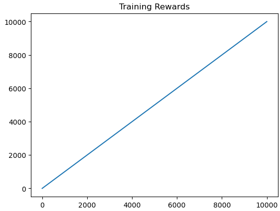
在此,我们使用 Matplotlib 根据经验回放缓冲区中的条目,通过绘制奖励随时间变化的趋势图来可视化训练性能。这有助于追踪智能体在训练过程中的累积奖励变化情况。
import matplotlib.pyplot as plt

plt.figure(figsize=(12, 6))
plt.plot(all_rewards)
plt.xlabel("Episode")
plt.ylabel("Total Reward")
plt.title("Training Performance")
plt.grid(True)
plt.show()
输出:
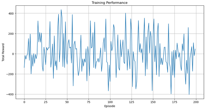
然后,我们通过绘制 all_rewards 来可视化智能体在各个回合中的表现,all_rewards 存储了每个回合中收集到的总奖励。该绘图通过网格和清晰的标签,便于阅读,展现了交易智能体随时间的学习进度和稳定性。
# Run a clean evaluation with the trained model (no exploration)
eval_env = TradingEnv(xau_data)
state = eval_env.reset()
eval_actions = []  # Store actions for this single episode

with torch.no_grad():
    while True:
        # Flatten state and predict
        state_tensor = torch.tensor(state, dtype=torch.float32).flatten().unsqueeze(0)
        q_values = model(state_tensor)
        action = q_values.argmax().item()

        next_state, _, done, _ = eval_env.step(action)
        eval_actions.append(action)
        state = next_state

        if done:
            break

# Now plot using eval_actions
close_prices = xau_data['<CLOSE>'].values
window_size = eval_env.observation_space.shape[0]

# Create action array with same length as price data
action_array = np.full(len(close_prices), np.nan)
action_array[window_size:window_size + len(eval_actions)] = eval_actions

# Create plot
plt.figure(figsize=(14, 8))
plt.plot(close_prices, label='XAUUSD Price', alpha=0.7)

# Plot buy signals (action=1)
buy_mask = (action_array == 1)
buy_indices = np.where(buy_mask)[0]
plt.scatter(buy_indices, close_prices[buy_mask],
            color='green', label='Buy', marker='^', s=100)

# Plot sell signals (action=2)
sell_mask = (action_array == 2)
sell_indices = np.where(sell_mask)[0]
plt.scatter(sell_indices, close_prices[sell_mask],
            color='red', label='Sell', marker='v', s=100)

plt.legend()
plt.title("Trading Actions on XAUUSD (Trained Policy)")
plt.xlabel("Time Step")
plt.ylabel("Price")
plt.grid(True)
plt.show()
输出:
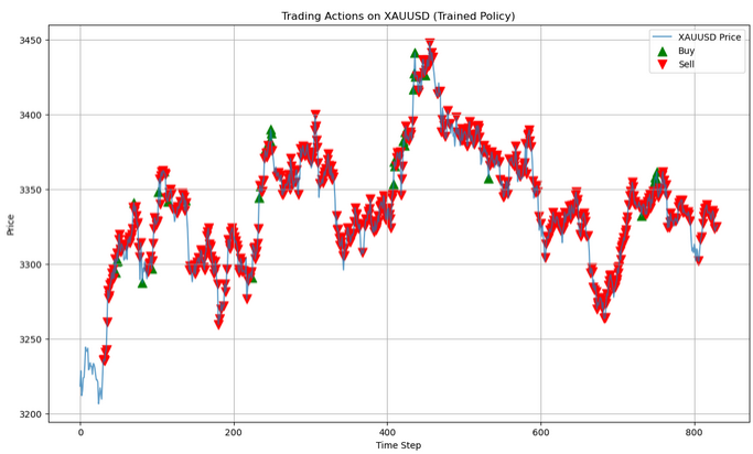
在此评估阶段,使用训练好的模型在不进行随机探索的评估环境(eval_env)中进行预测。智能体观察市场状态,根据其学习到的 Q 值选择最佳动作(贪婪地选择最高值),并记录所采取的每个动作。此循环持续进行,直至回合结束,使智能体能够在无随机性的情况下展示其学习到的策略。
dummy_input = torch.randn(1, *obs_shape)
torch.onnx.export(model, dummy_input, "dueling_dqn_xauusd.onnx",
                  input_names=["input"], output_names=["output"],
                  dynamic_axes={"input": {0: "batch_size"}, "output": {0: "batch_size"}}
最后,使用虚拟输入将训练好的对偶 DQN 模型导出为 ONNX 格式,以实现与其他平台的兼容性。这使得交易模型能够在 PyTorch 之外的环境中部署,例如实时系统或 MQL5 环境。
将所有内容放在 MQL5 中
//+------------------------------------------------------------------+
//|                                  ONNX_DQN_Trading_Script.mq5     |
//|                        Copyright 2023, MetaQuotes Ltd.           |
//|                                             https://www.mql5.com |
//+------------------------------------------------------------------+
#property copyright "Copyright 2023, MetaQuotes Ltd."
#property link      "https://www.mql5.com"
#property version   "1.00"
#property script_show_inputs

//--- input parameters
input string   ModelPath = "dueling_dqn_xauusd.onnx";  // File in MQL5\Files\
input int      WindowSize = 30;                        // Observation window size
input int      FeatureCount = 5;                       // Number of features

//--- ONNX model handle
long onnxHandle;

//--- Normalization parameters (REPLACE WITH YOUR ACTUAL VALUES)
const double   RSI_MEAN = 55.0,       RSI_STD = 15.0;
const double   MACD_MEAN = 0.05,      MACD_STD = 0.5;
const double   SMA20_MEAN = 1800.0,   SMA20_STD = 100.0;
const double   SMA50_MEAN = 1800.0,   SMA50_STD = 100.0;
const double   RETURN_MEAN = 0.0002,  RETURN_STD = 0.01;

//+------------------------------------------------------------------+
//| Script program start function                                    |
//+------------------------------------------------------------------+
void OnStart()
{
   //--- Load ONNX model
   onnxHandle = OnnxCreate(ModelPath, ONNX_DEFAULT);
   if(onnxHandle == INVALID_HANDLE)
   {
      Print("Error loading model: ", GetLastError());
      return;
   }

   //--- Prepare input data buffer
   double inputData[];
   ArrayResize(inputData, WindowSize * FeatureCount);

   //--- Collect and prepare data
   if(!PrepareInputData(inputData))
   {
      Print("Data preparation failed");
      OnnxRelease(onnxHandle);
      return;
   }

   //--- Set input shape (no need to set shape for dynamic axes)
   //--- Run inference
   double outputData[3];
   if(!RunInference(inputData, outputData))
   {
      Print("Inference failed");
      OnnxRelease(onnxHandle);
      return;
   }

   //--- Interpret results
   InterpretResults(outputData);
   OnnxRelease(onnxHandle);
}
//+------------------------------------------------------------------+
//| Prepare input data for the model                                 |
//+------------------------------------------------------------------+
bool PrepareInputData(double &inputData[])
{
   //--- Get closing prices
   double closes[];
   int closeCount = WindowSize + 1;
   if(CopyClose(_Symbol, _Period, 0, closeCount, closes) != closeCount)
   {
      Print("Not enough historical data. Requested: ", closeCount, ", Received: ", ArraySize(closes));
      return false;
   }

   //--- Calculate returns (percentage changes)
   double returns[];
   ArrayResize(returns, WindowSize);
   for(int i = 0; i < WindowSize; i++)
      returns[i] = (closes[i] - closes[i+1]) / closes[i+1];

   //--- Calculate technical indicators
   double rsi[], macd[], sma20[], sma50[];
   if(!CalculateIndicators(rsi, macd, sma20, sma50))
      return false;

   //--- Verify indicator array sizes
   if(ArraySize(rsi) < WindowSize || ArraySize(macd) < WindowSize ||
      ArraySize(sma20) < WindowSize || ArraySize(sma50) < WindowSize)
   {
      Print("Indicator data mismatch");
      return false;
   }

   //--- Normalize features and fill input data
   int dataIndex = 0;
   for(int i = WindowSize - 1; i >= 0; i--)
   {
      inputData[dataIndex++] = (rsi[i] - RSI_MEAN) / RSI_STD;
      inputData[dataIndex++] = (macd[i] - MACD_MEAN) / MACD_STD;
      inputData[dataIndex++] = (sma20[i] - SMA20_MEAN) / SMA20_STD;
      inputData[dataIndex++] = (sma50[i] - SMA50_MEAN) / SMA50_STD;
      inputData[dataIndex++] = (returns[i] - RETURN_MEAN) / RETURN_STD;
   }

   return true;
}
//+------------------------------------------------------------------+
//| Calculate technical indicators                                   |
//+------------------------------------------------------------------+
bool CalculateIndicators(double &rsi[], double &macd[], double &sma20[], double &sma50[])
{
   //--- RSI (14 period)
   int rsiHandle = iRSI(_Symbol, _Period, 14, PRICE_CLOSE);
   if(rsiHandle == INVALID_HANDLE) return false;
   if(CopyBuffer(rsiHandle, 0, 0, WindowSize, rsi) != WindowSize) return false;
   IndicatorRelease(rsiHandle);

   //--- MACD (12,26,9)
   int macdHandle = iMACD(_Symbol, _Period, 12, 26, 9, PRICE_CLOSE);
   if(macdHandle == INVALID_HANDLE) return false;
   double macdSignal[];
   if(CopyBuffer(macdHandle, 0, 0, WindowSize, macd) != WindowSize) return false;
   if(CopyBuffer(macdHandle, 1, 0, WindowSize, macdSignal) != WindowSize) return false;

   // Calculate MACD difference (histogram)
   for(int i = 0; i < WindowSize; i++)
      macd[i] = macd[i] - macdSignal[i];

   IndicatorRelease(macdHandle);

   //--- SMA20
   int sma20Handle = iMA(_Symbol, _Period, 20, 0, MODE_SMA, PRICE_CLOSE);
   if(sma20Handle == INVALID_HANDLE) return false;
   if(CopyBuffer(sma20Handle, 0, 0, WindowSize, sma20) != WindowSize) return false;
   IndicatorRelease(sma20Handle);

   //--- SMA50
   int sma50Handle = iMA(_Symbol, _Period, 50, 0, MODE_SMA, PRICE_CLOSE);
   if(sma50Handle == INVALID_HANDLE) return false;
   if(CopyBuffer(sma50Handle, 0, 0, WindowSize, sma50) != WindowSize) return false;
   IndicatorRelease(sma50Handle);

   return true;
}
//+------------------------------------------------------------------+
//| Run model inference                                              |
//+------------------------------------------------------------------+
bool RunInference(const double &inputData[], double &outputData[])
{
   //--- Run model directly without setting shape (for dynamic axes)
   if(!OnnxRun(onnxHandle, ONNX_DEBUG_LOGS, inputData, outputData))
   {
      Print("Model inference failed: ", GetLastError());
      return false;
   }
   return true;
}
//+------------------------------------------------------------------+
//| Interpret model results                                          |
//+------------------------------------------------------------------+
void InterpretResults(const double &outputData[])
{
   //--- Find best action
   int bestAction = ArrayMaximum(outputData);
   string actionText = "";

   switch(bestAction)
   {
      case 0: actionText = "HOLD"; break;
      case 1: actionText = "BUY"; break;
      case 2: actionText = "SELL"; break;
   }

   //--- Print results
   Print("Model Output: [HOLD: ", outputData[0], ", BUY: ", outputData[1], ", SELL: ", outputData[2], "]");
   Print("Recommended Action: ", actionText);
}
此 MQL5 脚本 ONNX_DQN_Trading_Script.mq5 旨在运行以 ONNX 格式导出的已训练的对偶 DQN 模型,以便在 MetaTrader 5 中生成交易信号。它首先从 Files 目录加载 ONNX 模型,并根据固定的观测窗口准备输入数据。它收集近期价格数据,计算 RSI、MACD 直方图、SMA20、SMA50 和收益率,再根据预定义的均值和标准差对这些特征进行标准化。这些处理后的特征被重塑为一维数组,以匹配模型预期的输入格式。
输入向量准备就绪后,脚本将使用 OnnxRun 进行推理,并返回三个输出值,这些值表示动作的预测 Q 值:HOLD(持有)、BUY(买入)、SELL(卖出)。具有最高值的操作被解释为模型的推荐,然后将其打印到终端上。推理步骤包含错误检查以确保稳健性,操作完成后会释放句柄以释放系统资源。
结论
总之,我们使用基于历史 XAUUSD 数据训练的对偶深度 Q 网络(Dueling DQN)架构,开发了一种自适应学习和灵活交易模型。该模型处理包括 RSI、MACD 直方图、SMA20、SMA50 和基于统计参数归一化的收益率百分比在内的技术特征滚动窗口。为确保学习稳定性,使用累积奖励对训练进度进行可视化。训练完成后,模型被导出为 ONNX 格式,以便集成到 MetaTrader 5 中,其中专用的 MQL5 脚本会加载模型,动态准备输入数据,运行推理,并根据最高输出概率解释模型的推荐操作(持有、买入或卖出)。
总之,这一端到端的流程为交易者提供了一个强大且自动化的决策支持系统,将深度强化学习与实时市场数据相结合。该系统的灵活性使得通过调整输入特征和重新训练,可以轻松适应新的交易品种或指标配置。通过将 ONNX 推理直接嵌入到 MQL5 中,交易者可以在其平台内部署智能模型,从而增强策略执行和市场响应能力,而无需依赖外部软件。
| 文件名称 | 描述 |
|---|---|
| Ada_flex.mq5 | 包含 MQL5 脚本的文件,该脚本作为在 Python 中训练的强化学习模型之间的桥梁 |
| Ada_L.ipynb | 包含用于训练模型并保存模型的 notebook 文件 |
| XAUUSD_H1.csv | 包含 XAUUSD 历史价格数据的文件 |
本文由MetaQuotes Ltd译自英文
原文地址: https://www.mql5.com/en/articles/18761
注意: MetaQuotes Ltd.将保留所有关于这些材料的权利。全部或部分复制或者转载这些材料将被禁止。
本文由网站的一位用户撰写,反映了他们的个人观点。MetaQuotes Ltd 不对所提供信息的准确性负责,也不对因使用所述解决方案、策略或建议而产生的任何后果负责。