计算机视觉在MQL5中的集成（第一部分）：构建基础函数

概述

屏幕微光闪烁，K线图勾勒出资金流动的轨迹，预示着一个全新交易时代的开启。您是否想过，当神经网络“审视”EURUSD市场时，它究竟“观察”到了什么？它如何解读每一次波动率的飙升、每一轮趋势的反转、每一个转瞬即逝的形态构建？

想象一台计算机，它不再机械地执行预设规则，而是真正地观察市场 —— 捕捉价格波动中那些人类肉眼无法察觉的微妙细节。正如经验丰富的船长能在风暴来临前察觉海平线气流的异动，这套AI系统也能以类似的方式解读EURUSD图表。

现在，我邀您共赴金融科技的最前沿，见证计算机视觉与市场分析的深度融合。我们将构建一个超越传统分析的系统 —— 它通过视觉理解市场，能像在人群中辨认挚友面容般自然地识别复杂价格形态。

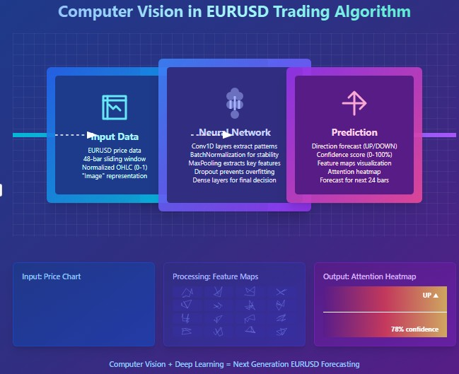
在毫秒决定千万命运的战场，我们的CNN模型为技术分析开辟了全新维度。它摒弃标准指标，直接从原始OHLC数据中学习并解析信号。最令人惊叹的是，我们得以窥探其“思维” —— 在做出决策前，哪些特定图表片段吸引了它的注意力。

计算机视觉模型的历史与应用

计算机视觉诞生于20世纪60年代的麻省理工学院（MIT），当时研究者首次尝试让机器解读视觉信息。初期进展缓慢：首批系统仅能识别简单形状与轮廓。

2012年迎来了真正的突破：深度卷积神经网络（CNN）的崛起彻底改变了行业格局。AlexNet架构在ImageNet竞赛中展现出前所未有的图像识别精度，由此开启了深度学习时代。

如今，计算机视觉正在重塑多个行业。在医疗领域，算法分析X光与MRI的准确度可媲美资深放射科医生。在汽车工业领域，驾驶辅助系统与自动驾驶通过计算机视觉识别道路物体。在智能手机技术领域，能够优化拍照效果并实现人脸解锁。在安防领域，系统通过面部识别实现门禁控制。

计算机视觉在金融分析中的应用尚属新兴领域，却充满潜力。计算机视觉算法能够识别传统技术指标无法捕捉的复杂图表形态，为算法交易开辟全新的视野。

技术基石：连接市场数据

我们的探索始于与市场的实时对话。如同神经末梢感知资金流动的脉搏，代码将接入MetaTrader 5终端 —— 这款经典交易工具如今已成为AI的门户：

import MetaTrader5 as mt5
import matplotlib
matplotlib.use('Agg')  # Using Agg backend for running without GUI
import matplotlib.pyplot as plt
from tensorflow.keras.models import Sequential, Model
from tensorflow.keras.layers import Dense, Conv1D, MaxPooling1D, Flatten, Dropout, BatchNormalization, Input

# Connecting to MetaTrader5 terminal
def connect_to_mt5():
    if not mt5.initialize():
        print("Error initializing MetaTrader5")
        mt5.shutdown()
        return False
    return True

代码的起始几行，象征着算法世界与金融领域的正式连接。这看似简单的函数调用，实则开辟了一条数据通道 —— 全球数百万交易者决策交汇形成的报价、以GB为单位的市场数据，将在此川流不息。

我们的系统采用无图形用户界面（GUI）的Agg渲染后端进行可视化。这个看似细节的设计，却让系统能在远程服务器后台持续运行，对市场的每一秒波动都保持毫秒级响应的警惕。

溯源历史：数据采集与预处理

所有AI的起点都是数据。对我们而言，这些数据是数千根EURUSD小时K线 —— 它们是过去价格博弈的无声见证者，蕴藏着等待被破译的形态密码：

def get_historical_data(symbol="EURUSD", timeframe=mt5.TIMEFRAME_H1, num_bars=1000):
    now = datetime.now()
    from_date = now - timedelta(days=num_bars/24)  # Approximate for hourly bars
    
    rates = mt5.copy_rates_range(symbol, timeframe, from_date, now)
    if rates is None or len(rates) == 0:
        print("Error loading historical quotes")
        return None
    
    # Convert to pandas DataFrame
    rates_frame = pd.DataFrame(rates)
    rates_frame['time'] = pd.to_datetime(rates_frame['time'], unit='s')
    rates_frame.set_index('time', inplace=True)
    
    return rates_frame

此函数是第一个"魔法"发生之处：原始字节流在此转化为有序的数据。每一根K线、每一次价格波动，都化作多维空间中的坐标点，等待神经网络去探索其中的规律。我们加载2000根历史K线。这个数量足以让模型捕捉从平静趋势到剧烈波动时期的各类市场状态。

但计算机视觉需要的不仅是数字，更是图像。接下来的关键步骤，是将时间序列转化为卷积网络能够解析的“图像”：

def create_images(data, window_size=48, prediction_window=24):
    images = []
    targets = []
    
    # Using OHLC data to create images
    for i in range(len(data) - window_size - prediction_window):
        window_data = data.iloc[i:i+window_size]
        target_data = data.iloc[i+window_size:i+window_size+prediction_window]
        
        # Normalize data in the window
        scaler = MinMaxScaler(feature_range=(0, 1))
        window_scaled = scaler.fit_transform(window_data[['open', 'high', 'low', 'close']])
        
        # Predict price direction (up/down) for the forecast period
        price_direction = 1 if target_data['close'].iloc[-1] > window_data['close'].iloc[-1] else 0
        
        images.append(window_scaled)
        targets.append(price_direction)
    
    return np.array(images), np.array(targets)

这就像是一次数据“炼金”。我们将48根连续价格K线作为时间窗口，将数值标准化至0-1区间，并转化为多通道图像 —— 每个通道对应开盘价（O）、最高价（H）、最低价（L）、收盘价（C）中的一个分量。对于每一帧的市场历史“切片”，我们确定一个目标值 —— 未来24根K线的价格方向。

滑动窗口如精密齿轮般遍历整个数据集，生成数千个训练样本。这恰似一位资深交易员逐帧翻阅历史图表，在价格形态中捕捉规律，学会识别重大行情爆发前的信号特征。

打造神经之“眼”：模型架构设计

现在，让我们继续构建合适的神经网络。这双人工之眼将穿透市场数据的混沌，寻找隐匿的秩序。我们的架构借鉴了计算机视觉领域的最新突破，但针对金融时间序列的特性进行了深度定制：

def train_cv_model(images, targets):
    # Split data into training and validation sets
    X_train, X_val, y_train, y_val = train_test_split(images, targets, test_size=0.2, shuffle=True, random_state=42)
    
    # Create model with improved architecture
    inputs = Input(shape=X_train.shape[1:])
    
    # First convolutional block
    x = Conv1D(filters=64, kernel_size=3, padding='same', activation='relu')(inputs)
    x = BatchNormalization()(x)
    x = Conv1D(filters=64, kernel_size=3, padding='same', activation='relu')(x)
    x = BatchNormalization()(x)
    x = MaxPooling1D(pool_size=2)(x)
    x = Dropout(0.2)(x)
    
    # Second convolutional block
    x = Conv1D(filters=128, kernel_size=3, padding='same', activation='relu')(x)
    x = BatchNormalization()(x)
    x = Conv1D(filters=128, kernel_size=3, padding='same', activation='relu')(x)
    x = BatchNormalization()(x)
    x = MaxPooling1D(pool_size=2)(x)
    feature_maps = x  # Store feature maps for visualization
    x = Dropout(0.2)(x)
    
    # Output block
    x = Flatten()(x)
    x = Dense(128, activation='relu')(x)
    x = BatchNormalization()(x)
    x = Dropout(0.3)(x)
    x = Dense(64, activation='relu')(x)
    x = BatchNormalization()(x)
    x = Dropout(0.3)(x)
    outputs = Dense(1, activation='sigmoid')(x)
    
    # Create the full model
    model = Model(inputs=inputs, outputs=outputs)
    
    # Create a feature extraction model for visualization
    feature_model = Model(inputs=model.input, outputs=feature_maps)

我们采用Keras函数式API而非顺序模型。这赋予我们构建辅助模型的灵活性 —— 可提取中间层特征用于可视化分析。这正是该方法的核心创新所在：我们不仅构建预测系统，更创造了一面窥视AI“思维”的镜子。

模型架构由两个卷积模块组成，每个模块包含两个带批量标准化的卷积层。第一模块使用64个滤波器，第二模块使用128个滤波器，逐层揭示更复杂的市场模式。完成特征提取后，数据流经全连接层进行信息整合，最终输出未来价格方向的预测概率。

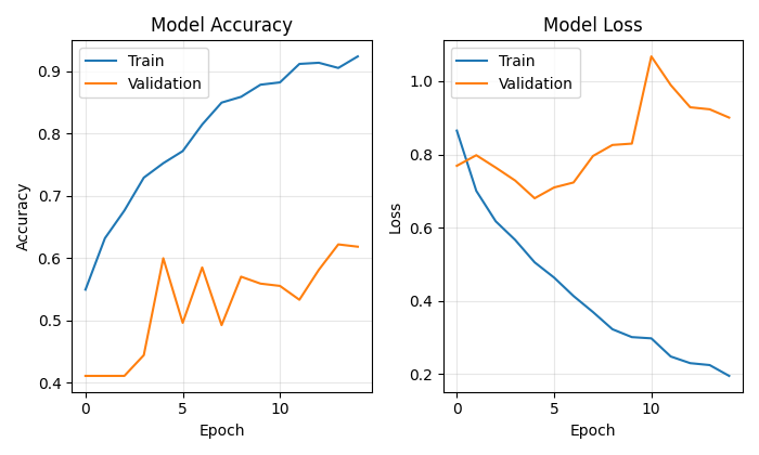
训练模型不仅仅是优化损失函数， 更是一场穿越参数空间的探索，每次迭代都让我们离目标更近一步：

# Early stopping to prevent overfitting
early_stopping = EarlyStopping(
    monitor='val_loss',
    patience=10,
    restore_best_weights=True,
    verbose=1
)

# Train model
history = model.fit(
    X_train, y_train,
    epochs=50,
    batch_size=32,
    validation_data=(X_val, y_val),
    callbacks=[early_stopping],
    verbose=1
)

我们采用早停法防止过拟合 —— 当模型在验证集上的表现不再提升时，神经网络将自动终止训练。这帮助我们在欠拟合与过拟合之间找到黄金平衡点，实现最佳泛化能力。

窥视AI的“思维”

此方法的独特之处在于，它能直观地展示模型是如何“观察”市场的。通过两项创新功能，我们得以揭开神经网络的神秘面纱：

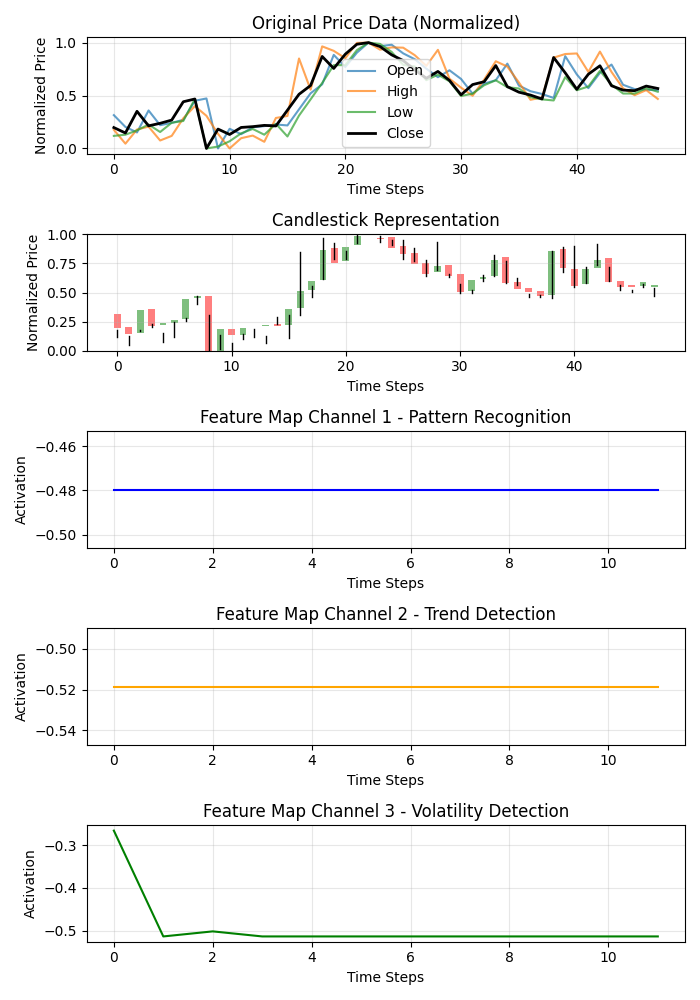
def visualize_model_perception(feature_model, last_window_scaled, window_size=48):
    # Get feature maps for the last window
    feature_maps = feature_model.predict(np.array([last_window_scaled]))[0]
    
    # Plot feature maps
    plt.figure(figsize=(7, 10))
    
    # Plot original data
    plt.subplot(5, 1, 1)
    plt.title("Original Price Data (Normalized)")
    plt.plot(np.arange(window_size), last_window_scaled[:, 0], label='Open', alpha=0.7)
    plt.plot(np.arange(window_size), last_window_scaled[:, 1], label='High', alpha=0.7)
    plt.plot(np.arange(window_size), last_window_scaled[:, 2], label='Low', alpha=0.7)
    plt.plot(np.arange(window_size), last_window_scaled[:, 3], label='Close', color='black', linewidth=2)
    
    # Plot candlestick representation
    plt.subplot(5, 1, 2)
    plt.title("Candlestick Representation")
    
    # Width of the candles
    width = 0.6
    
    for i in range(len(last_window_scaled)):
        # Candle color
        if last_window_scaled[i, 3] >= last_window_scaled[i, 0]:  # close >= open
            color = 'green'
            body_bottom = last_window_scaled[i, 0]  # open
            body_height = last_window_scaled[i, 3] - last_window_scaled[i, 0]  # close - open
        else:
            color = 'red'
            body_bottom = last_window_scaled[i, 3]  # close
            body_height = last_window_scaled[i, 0] - last_window_scaled[i, 3]  # open - close
        
        # Candle body
        plt.bar(i, body_height, bottom=body_bottom, color=color, width=width, alpha=0.5)
        
        # Candle wicks
        plt.plot([i, i], [last_window_scaled[i, 2], last_window_scaled[i, 1]], color='black', linewidth=1)
    
    # Plot feature maps visualization (first 3 channels)
    plt.subplot(5, 1, 3)
    plt.title("Feature Map Channel 1 - Pattern Recognition")
    plt.plot(time_indices, feature_maps[:, 0], color='blue')
    
    plt.subplot(5, 1, 4)
    plt.title("Feature Map Channel 2 - Trend Detection")
    plt.plot(time_indices, feature_maps[:, 1], color='orange')
    
    plt.subplot(5, 1, 5)
    plt.title("Feature Map Channel 3 - Volatility Detection")
    plt.plot(time_indices, feature_maps[:, 2], color='green')

该函数生成多面板可视化图，同步展示原始数据序列、K线图形态和卷积滤波器前三个通道的激活热力图。每个通道专注于市场动态的特定方面：一个捕捉重复模式，另一个关注趋势，剩下的第三个对波动性做出反应。如同揭示资深交易员大脑不同区域的专业化分工。

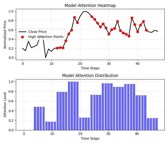
注意力热图带来更惊喜的发现：

def visualize_attention_heatmap(feature_model, last_window_scaled, window_size=48):
    # Get feature maps for the last window
    feature_maps = feature_model.predict(np.array([last_window_scaled]))[0]
    
    # Average activation across all channels to get a measure of "attention"
    avg_activation = np.mean(np.abs(feature_maps), axis=1)
    
    # Normalize to [0, 1] for visualization
    attention = (avg_activation - np.min(avg_activation)) / (np.max(avg_activation) - np.min(avg_activation))
    
    # Upsample attention to match original window size
    upsampled_attention = np.zeros(window_size)
    ratio = window_size / len(attention)
    
    for i in range(len(attention)):
        start_idx = int(i * ratio)
        end_idx = int((i+1) * ratio)
        upsampled_attention[start_idx:end_idx] = attention[i]
    
    # Plot the heatmap
    plt.figure(figsize=(7, 6))
    
    # Price plot with attention heatmap
    plt.subplot(2, 1, 1)
    plt.title("Model Attention Heatmap")
    
    # Plot close prices
    time_indices = np.arange(window_size)
    plt.plot(time_indices, last_window_scaled[:, 3], color='black', linewidth=2, label='Close Price')
    
    # Add shading based on attention
    plt.fill_between(time_indices, last_window_scaled[:, 3].min(), last_window_scaled[:, 3].max(), 
                     alpha=upsampled_attention * 0.5, color='red')
                     
    # Highlight points with high attention
    high_attention_threshold = 0.7
    high_attention_indices = np.where(upsampled_attention > high_attention_threshold)[0]
    plt.scatter(high_attention_indices, last_window_scaled[high_attention_indices, 3], 
               color='red', s=50, zorder=5, label='High Attention Points')

该功能绘制出模型“思维”的实时图谱，揭示K线图中哪些区域对预测结果影响最大。高关注度红色区域往往精准覆盖关键价位与反转点，印证了模型已学会自主识别重要价格形态。

从预测到盈利：实战转化

系统的终极环节，是将复杂的预测转化为交易员可理解的决策信号：

def plot_prediction(data, window_size=48, prediction_window=24, direction="UP ▲"):
    plt.figure(figsize=(7, 4.2))
    
    # Get the last window of data for visualization
    last_window = data.iloc[-window_size:]
    
    # Create time index for prediction
    last_date = last_window.index[-1]
    future_dates = pd.date_range(start=last_date, periods=prediction_window+1, freq=data.index.to_series().diff().mode()[0])[1:]
    
    # Plot closing prices
    plt.plot(last_window.index, last_window['close'], label='Historical Data')
    
    # Add marker for current price
    current_price = last_window['close'].iloc[-1]
    plt.scatter(last_window.index[-1], current_price, color='blue', s=100, zorder=5)
    plt.annotate(f'Current price: {current_price:.5f}', 
                 xy=(last_window.index[-1], current_price),
                 xytext=(10, -30),
                 textcoords='offset points',
                 fontsize=10,
                 arrowprops=dict(arrowstyle='->', color='black'))
    
    # Visualize the predicted direction
    arrow_start = (last_window.index[-1], current_price)
    
    # Calculate range for the arrow (approximately 10% of price range)
    price_range = last_window['high'].max() - last_window['low'].min()
    arrow_length = price_range * 0.1
    
    # Up or down prediction
    if direction == "UP ▲":
        arrow_end = (future_dates[-1], current_price + arrow_length)
        arrow_color = 'green'
    else:
        arrow_end = (future_dates[-1], current_price - arrow_length)
        arrow_color = 'red'
    
    # Direction arrow
    plt.annotate('', 
                 xy=arrow_end,
                 xytext=arrow_start,
                 arrowprops=dict(arrowstyle='->', lw=2, color=arrow_color))
    
    plt.title(f'EURUSD - Forecast for {prediction_window} periods: {direction}')

该可视化图表将抽象的预测结果转化为直观的交易信号。绿色箭头表示预期上涨，红色箭头表示预期下跌。交易员可瞬间掌握当前局势，并获得AI分析支撑的决策依据。

但我们的系统不止于预测方向。还提供预测置信度的量化评估。

# Predict on the last available window
def make_prediction(model, data, window_size=48):
    # Get the last window of data
    last_window = data.iloc[-window_size:][['open', 'high', 'low', 'close']]
    
    # Normalize data
    scaler = MinMaxScaler(feature_range=(0, 1))
    last_window_scaled = scaler.fit_transform(last_window)
    
    # Prepare data for the model
    last_window_reshaped = np.array([last_window_scaled])
    
    # Get prediction
    prediction = model.predict(last_window_reshaped)[0][0]
    
    # Interpret result
    direction = "UP ▲" if prediction > 0.5 else "DOWN ▼"
    confidence = prediction if prediction > 0.5 else 1 - prediction
    
    return direction, confidence * 100, last_window_scaled

神经网络的输出值不再被简单地解读为二元答案，而是转化为上涨概率值。这样使交易员能够做出更理性的决策 —— 不仅考虑方向，还综合评估系统对预测的置信度。例如，置信度为95%的预测可以支持更激进的策略，而置信度为55%的预测则需谨慎操作。

调度流程：主函数

将所有系统模块整合至主函数中，实现从数据接入到结果可视化的整个流程：

def main():
    print("Starting EURUSD prediction system with computer vision")
    
    # Connect to MT5
    if not connect_to_mt5():
        return
    
    print("Successfully connected to MetaTrader5")
    
    # Load historical data
    bars_to_load = 2000  # Load more than needed for training
    data = get_historical_data(num_bars=bars_to_load)
    if data is None:
        mt5.shutdown()
        return
    
    print(f"Loaded {len(data)} bars of EURUSD history")
    
    # Convert data to image format
    print("Converting data for computer vision processing...")
    images, targets = create_images(data)
    print(f"Created {len(images)} images for training")
    
    # Train model
    print("Training computer vision model...")
    model, history, feature_model = train_cv_model(images, targets)
    
    # Visualize training process
    plot_learning_history(history)
    
    # Prediction
    direction, confidence, last_window_scaled = make_prediction(model, data)
    print(f"Forecast for the next 24 periods: {direction} (confidence: {confidence:.2f}%)")
    
    # Visualize prediction
    plot_prediction(data, direction=direction)
    
    # Visualize how the model "sees" the market
    visualize_model_perception(feature_model, last_window_scaled)
    
    # Visualize attention heatmap
    visualize_attention_heatmap(feature_model, last_window_scaled)
    
    # Disconnect from MT5
    mt5.shutdown()
    print("Work completed")

该函数如同指挥家一般，统筹调度着数据与算法的复杂流程。它带领我们一步步穿越整个流程 —— 从终端的首次数据连接，到最终揭开AI内心世界的可视化呈现。

结论：算法交易的新纪元

我们构建的不仅是又一个技术指标或交易系统。而是用计算机视觉重构市场认知的全新模式，使我们突破人类视觉的局限，在价格波动的噪声中捕捉隐藏的规律。

这绝不仅仅是一个输出神秘信号的黑盒子。借助可视化技术，我们可以观察模型如何感知市场、关注价格变化的哪些特征，以及如何生成预测。这在交易者与算法之间架起了信任的桥梁。

当高频算法以每秒百万笔的速度执行交易时，我们的系统代表着截然不同的深度交易哲学 —— 不追求执行速度，而是通过计算机视觉的透镜，解析市场动态的本质规律。

代码开源，技术普惠，成果斐然。您踏入计算机视觉交易世界的旅程，此刻才刚刚启程。或许正是通过神经网络的算法棱镜，您将观察到此前不可见的真相，找到破解汇率报价变幻之舞的密钥。

想象未来的交易场景：您的屏幕上不再只有传统K线与指标线，而是实时呈现AI感知的市场形势 —— 突出哪些模式，以及需要特别关注哪些价格水平。这不再是科幻场景。而是如今可用的技术。迈出这一步，您将开启算法交易的新纪元。