重塑经典策略（第三部分）：预测新高与新低

引言

人工智能为交易能力的提升提供了近乎无限的可能。但并非所有策略都能奏效。我们的目标是通过提供决策所需的关键信息，帮助交易者筛选最适合自身需求的策略方案。

面对海量的策略组合可能性，任何交易者都难以在重大决策前完成全面评估。这是整个交易社群共同面临的痛点。因此，本系列文章将通过对比经典策略与基础模型的预测精度，系统探索交易策略的优化空间。

本文深入剖析了基于"更高高点/更低低点"的经典价格行为策略。我们训练了多种模型来预测两个差异化目标。基础目标是预测价格变动方向。进阶目标则是预判未来收盘价会突破当前极值（高于现高点或低于现低点），还是维持区间震荡。

为了比较不同复杂度的模型，我们采用了时间序列交叉验证，而未进行随机打乱。我们分析了两个目标上准确率分数的变化。结果表明，预测价格变动方向的简约模型可能更具实效价值。

交易策略概览

当采用价格行为策略的交易者分析某一标的时，他们通常会寻找强势趋势正在形成或即将消亡的迹象。一个众所周知的强势趋势正在形成的迹象是，价格水平收盘价高于先前的极端值，并继续以逐渐增大的步幅远离这些极端值。这俗称“新高”或“新低”，具体取决于价格移动的方向。

无数代的交易者都使用了这一简单策略来确定入场和出场点。出场点通常是在价格未能突破其极端值时确定的，这表明趋势正在减弱，并可能潜在反转。多年来，该策略虽然增加了一些小的扩展，但其基本模板始终保持不变。

该策略最大的缺点之一是，价格意外地回落到其极端值以下。这些不利的价格变动被称为“回调”，且难以预测。因此，大多数交易者不会在价格突破新的极端值时立即入场。反，他们会等待观察价格能否维持在这些水平之上一段时间后再做决定——这本质上是在让趋势自我证明。然而，这种方法引发了几个问题：要等待多久才能断定趋势已经得到证明？相反，趋势反转之前等待太久是否也不合适？这是价格行为分析师所面临的困境。

方法论概述

既然我们已经了解了这种交易策略的弱点，我们就明白了采用人工智能来克服这些过去限制的动机。如前所述，我们训练了一组多样化的分类器来预测价格是否会收盘价高于其当前的极端值或保持在当前范围内。我们为此任务选择了各种分类器，包括AdaBoost、决策树和神经网络。在比较之前，我们没有对任何模型进行超参数调整。

我们将三种可能的结果映射到三个类别级别：1、2和3，分别代表：

• 1表示未来收盘价将高于现在的最高价；
• 2表示未来收盘价将低于现在的最低价；
• 3表示1和2都不正确，未来价格将在当前最高价和最低价之间。

值得注意的是，我们创建的新目标更难解释。如果我们的模型预测将过渡到状态3，那么根据当时的价格，价格水平是上涨还是下跌可能仍不确定。这使得我们的模型不仅透明度更低，而且表面上看似比最简单的模型准确性也更低。
通常，我们会给任何能够超越最简单模型的策略以认可。一个未能做到这一点的复杂策略可能无法证明其对有限资源（如时间）的额外投入是合理的。

Python中的探索性数据分析

为了开始，我们首先需要从MetaTrader 5终端导出市场数据。我们首先打开终端，选择“Symbol”图标。然后从上下文菜单中选择“bars”，搜索你感兴趣的符号，然后按“export”导出。

图1：准备导出市场数据

既然我们的数据已经准备就绪，接下来让我们开始可视化，看看所讨论的变量之间是否存在任何关系。

首先，我们需要导入所需的库。

#import libraries
import pandas as pd
import numpy as np
import seaborn as sns
import matplotlib.pyplot as plt

接着，我们读取之前准备的数据。请注意，MetaTrader 5终端提供的是以制表符分隔的csv文件。因此，在读取文件时，我们需要传递“\t”参数来指定制表符作为分隔符。

gbpusd = pd.read_csv("/home/volatily/market_data/GBPUSD_Daily_20160103_20240131.csv",sep="\t")

让我们将列数据重命名

#Rename the columns
gbpusd.rename(columns={"<DATE>":"Date","<OPEN>":"Open","<HIGH>":"High","<LOW>":"Low","<CLOSE>":"Close","<TICKVOL>":"TickVol","<VOL>":"Vol","<SPREAD>":"Spread"},inplace=True)

让我们确定我们想要预测多远的未来。

#Define how far into the future we want to forecast
look_ahead = 20

现在，我们将以之前讨论过的方式定义我们的标签。

#This column will help us with our plots
gbpusd["Future Close"] = gbpusd["Close"].shift(-look_ahead)
#Let's mark the normal target
#If price rises, our target will be 1
#If price falls, our target will be 0
gbpusd["Price Target"] = 0
#Let's mark the new target
#If price makes a higher high, we will label 1
#If price makes a lower low, we will label 2
#If price fails to make either, we will label 3
gbpusd["New Target"] = 0

对数据进行标记。

#Labeling the data
#If the future close was less than the current close, price depreciated, label 0
gbpusd.loc[gbpusd["Close"] > gbpusd["Close"].shift(-look_ahead),"Price Target"] = 0
#If the future close was greater than the current close, price depreciated, label 1
gbpusd.loc[gbpusd["Close"] < gbpusd["Close"].shift(-look_ahead),"Price Target"] = 1
#If price makes a higher high our label will be 1
gbpusd.loc[gbpusd["Close"].shift(-look_ahead) > gbpusd["High"],"New Target"] = 1
#If price makes a lower low our label will be 2
gbpusd.loc[gbpusd["Close"].shift(-look_ahead) < gbpusd["Low"],"New Target"] = 2
#Otherwise our label will be 3 
gbpusd.loc[gbpusd["Close"].shift(-look_ahead) < gbpusd["Low"],"New Target"] = 3

我们可以删除所有包含缺失值的行。

#Drop the last look ahead rows
gbpusd = gbpusd[:-look_ahead]

交易策略暗示收盘价和最高价之间存在某种关系，让我们来可视化收盘价和最高价之间是否存在这种关系。

#Plot a scattor plot so we can see if there may be any relationship between the close and the high
sns.scatterplot(data=gbpusd,x="Close",y="High",hue="Price Target")

图2：收盘价对最高价的图形化展示

散点图很有帮助，因为它们允许我们可视化我们正在建模的系统中任何一对状态变量之间的关系。
通过观察数据，我们可以立即看到收盘价和最高价之间似乎存在强烈且几乎线性的关系。为了给图表增加可读性，我们为图表添加了颜色，以区分价格上涨和价格下跌的情况。然而，我们观察到这两种情况之间并没有明显的分离。唯一明显的分离点出现在极端值处；例如，当收盘价低于1.1水平时，它似乎总是会反弹。

我们可以再次绘制相同的散点图，但这次我们将最低价放在y轴上。

#Plot a scattor plot so we can see if there may be any relationship between the close and the low
sns.scatterplot(data=gbpusd,x="Close",y="Low",hue="Price Target")

图3：收盘价与最低价关系的图形化展示

正如预期，我们没有得到太多的自然离散点。这种自然分离是我们所期望的，因为它能帮助我们的模型更快地学习到决策边界。让我们看看我们的新目标是否能帮助我们更好地分离数据集。

#Plot a scattor plot so we can see if there may be any relationship between the close and the low
sns.scatterplot(data=gbpusd,x="Close",y="Low",hue="New Target")

图4：我们的新目标并没有带来更多的离散点

如我们所见，离散点仍旧很少。最暗的点，代表状态3，几乎贯穿了我们整个图表的整个长度。这是有问题的，因为从图中表明，在我们的数据中，存在相同的输入导致不同输出的情况。
为了展示良好的离散形态是什么样子，让我们将当前价格放在x轴上，未来价格放在y轴上进行图形化。我们将价格上涨的图表点着色为橙色，价格下跌的着色为蓝色。

#Plot a scattor plot so we can see if there may be any relationship between the close and the low
sns.scatterplot(data=gbpusd,x="Close",y="Future Close",hue="Price Target")

图5：良好的分离形态的一个示例

如您所见，在这个图中，两类之间有明显的分离。这是可以预料的，因为我们在图中使用了目标本身。作为机器学习从业者，我们的目标是找到一个特征或目标，它能给我们提供接近图4中所示程度的分离。

如果我们使用新的目标进行相同的绘图，我们会观察到一些奇特的现象。

#Plot a scattor plot so we can see if there may be any relationship between the close and the low
sns.scatterplot(data=gbpusd,x="Close",y="Future Close",hue="New Target")

图6：新目标的分离形态图

观察发现，在图表的上半部分和下半部分，深色点和浅色点被很好地分开，分别代表了价格上涨和价格下跌的情况。在这两类之间，我们有被分类为状态3的点，它们由沿中心分布的暗点表示，显示了价格处于波动范围的情况。

训练模型

现在，我们将导入所需的模型和其他预处理工具。

#Let's get a group of different models
from sklearn.ensemble import RandomForestClassifier
from sklearn.ensemble import BaggingClassifier
from sklearn.ensemble import AdaBoostClassifier
from sklearn.neighbors import KNeighborsClassifier
from sklearn.discriminant_analysis import LinearDiscriminantAnalysis
from sklearn.neural_network import MLPClassifier
from sklearn.svm import LinearSVC
#Import cross validation libraries
from sklearn.model_selection import TimeSeriesSplit
#Import accuracy metrics
from sklearn.metrics import accuracy_score
#Import preprocessors
from sklearn.preprocessing import RobustScaler

我们将为我们的时间序列交叉验证定义参数。请记住，间隔应至少等于我们的预测范围。

#Splits
splits = 10
gap = look_ahead

让我们将所需的每个模型存储在一个列表中，以便我们可以编程拟合我们所有的模型。

#Store each of the models we need
cols = ["AdaBoostClassifier","Linear DiscriminantAnalysis","Bagging Classifier","Random Forest Classifier","KNeighborsClassifier","Neural Network Small","Neural Network Large"]
models = [AdaBoostClassifier(),LinearDiscriminantAnalysis(),BaggingClassifier(n_jobs=-1),RandomForestClassifier(n_jobs=-1),KNeighborsClassifier(n_jobs=-1),MLPClassifier(hidden_layer_sizes=(5,2),early_stopping=True,max_iter=1000),MLPClassifier(hidden_layer_sizes=(20,10),early_stopping=True,max_iter=1000)]
#Create data frames to store our accuracy with different models on different targets
index = np.arange(0,splits)
price_target = pd.DataFrame(columns=cols,index=index)
new_target = pd.DataFrame(columns=cols,index=index)

我们将为交叉验证测试创建时间序列分离对象。

#Create the tscv splits
tscv = TimeSeriesSplit(n_splits=splits,gap=gap)

让我们为我们的模型定义预测变量和目标变量。

#Define the predictors and target
predictors = ["Open","High","Low","Close"]
target = "New Target"

执行交叉验证。

#Now we perform cross validation
for j in (np.arange(len(models))):
    #We need to train each model
    model = models[j]
    for i,(train,test) in enumerate(tscv.split(gbpusd)):
        #Scale the data
        scaler = RobustScaler()
        X_train_scaled = scaler.fit_transform(gbpusd.loc[train[0]:train[-1],predictors])
        scaler = RobustScaler()
        X_test_scaled = scaler.fit_transform(gbpusd.loc[test[0]:test[-1],predictors])
        #Train the model
        model.fit(X_train_scaled,gbpusd.loc[train[0]:train[-1],target])
        #Measure the accuracy
        new_target.iloc[i,j] = accuracy_score(gbpusd.loc[test[0]:test[-1],target],model.predict(X_test_scaled))

让我们观察每个模型在最简单目标上的表现。

#Calculate the mean for each column when predicting price 
for i in np.arange(0,len(models)):
    print(f"{cols[i]} achieved accuracy: {price_target.iloc[:,i].mean()}")

AdaBoostClassifier 获得的准确度为：0.5190265486725664
Linear Discriminant Analysis 获得的准确度为：0.5579646017699115
Bagging Classifier 获得的准确度为：0.5075221238938052
Random Forest Classifier 获得的准确度为：0.5349557522123894
KNeighborsClassifier 获得的准确度为：0.536283185840708
Neural Network Small 获得的准确度为：0.45309734513274336
Neural Network Large 获得的准确度为：0.5446902654867257

线性判别分析（LDA）在这个特定数据集上表现最佳，几乎达到了56%的准确率。但让我们现在看看我们在新目标上的表现。

#Calculate the mean for each column when predicting price 
for i in np.arange(0,len(models)):
    print(f"{cols[i]} achieved accuracy: {new_target.iloc[:,i].mean()}")

AdaBoostClassifier 获得的准确度为：0.45929203539823016
Linear DiscriminantAnalysis 获得的准确度为：0.4668141592920355
Bagging Classifier 获得的准确度为：0.4393805309734514
Random Forest Classifier 获得的准确度为：0.45929203539823016
KNeighborsClassifier 获得的准确度为：0.465929203539823
Neural Network Small 获得的准确度为：0.3920353982300885
Neural Network Large 获得的准确度为：0.4606194690265487

在两个例子中LDA的表现都排名前列。所有模型在新目标上的表现都较弱，但小型神经网络模型的性能下降幅度最大。

模型	表现的变化
AdaBoostClassifier	-14.32748538011695%
Linear Discriminant Analysis	-19.526066350710863%
Bagging Classifier	-22.09660842754366%
Random Forest Classifier	-16.730769230769248%
KNeighborsClassifier	-15.099715099715114%
Neural Network Small	-41.04193138500632%
Neural Network Large	-21.1502782931354%

让我们来分析我们表现最好的模型的混淆矩阵。

#Let's continue analysing the performance of our best model Linear Discriminant Analysis
from mlxtend.evaluate import confusion_matrix
from mlxtend.plotting import plot_confusion_matrix
model = LinearDiscriminantAnalysis()
model.fit(gbpusd.loc[0:1000,predictors],gbpusd.loc[0:1000,"New Target"])
cm = confusion_matrix(y_target=gbpusd.loc[1000:,"New Target"],y_predicted=model.predict(gbpusd.loc[1000:,predictors]),binary=True)
fig , ax = plot_confusion_matrix(cm)

图7：LDA模型的混淆矩阵

混淆矩阵是一个有力的工具，它能帮助我们识别出哪些类别对模型来说更具挑战性。如上图所示，在预测第3类时，我们的模型表现最差。然而，这个类别的观测数据较少。为了解决这个问题，我们可能需要使用更能代表整体群体的数据。这可以通过获取更多的历史数据或分析更低的时间框架来实现。

特征选择

有时，通过从模型中剔除不必要的特征，我们可以提升性能。让我们聚焦于表现最佳的线性判别分析（LDA）模型，并确定其最重要的特征，看看是否还能进一步提升性能。

#Now let us perform feature selection
from mlxtend.feature_selection import SequentialFeatureSelector

特征选择算法众多，而本文中我们采用了前向特征选择算法。尽管该算法有多个版本，但一般流程都是从一个作为基准的空模型开始。然后，算法逐一评估p个可用特征，并选择能带来最大性能提升的特征作为第一个特征。这个过程会对剩下的p-1个预测变量重复进行。得益于近年来并行计算的飞速发展，此类算法已变得更加可行。

通过从p个预测变量中减少到k个（其中k<p），并明智地选择这k个特征，我们或许能够超越原始模型的性能，或者获得一个同样可靠但训练速度更快的模型。此外，减少模型中使用的预测变量数量还可以降低模型系数的方差。

然而，该算法存在两个值得探讨的显著局限性。首先，由于我们用于训练模型的信息有限，新模型可能会产生更大的偏差。此外，第一个特征的选择会影响后续的选择。如果最初选择的特征与目标关系不大，那么由于这个糟糕的初始选择，后续的特征可能会显得缺乏信息量。

在我们的分析中，我们允许特征选择器选择它认为重要的任意数量的变量，但它只选择了一个：开盘价。

#Forward feature selection 
forward_feature_selection = SequentialFeatureSelector(LinearDiscriminantAnalysis(),
                                                     k_features =(1,4),
                                                     forward=True,
                                                     verbose=2,
                                                     scoring="accuracy",
                                                     cv=5,
                                                     n_jobs=-1).fit(gbpusd.loc[:,predictors],gbpusd.loc[:,"New Target"])

现在我们想要得到最佳特征。

#Best feature
forward_feature_selection.k_feature_names_

(Open,)

让我们观察最新的准确度。

#Update the predictors and target
predictors = ["Open"]
target = "New Target"
best_features_for_new_target = pd.DataFrame(columns=["Linear Discriminant Analysis"],index=index)

使用我们确定的最佳特征进行交叉验证。

#Now we perform cross validation
for i,(train,test) in enumerate(tscv.split(gbpusd)):
    #First initialize the model
    model = LogisticRegression()
    #Train the model
    model.fit(gbpusd.loc[train[0]:train[-1],predictors],gbpusd.loc[train[0]:train[-1],target])
    #Measure the accuracy
    best_features_for_new_target.iloc[i,0] = accuracy_score(gbpusd.loc[test[0]:test[-1],target],model.predict(gbpusd.loc[test[0]:test[-1],predictors]))

让我们观察最新的准确度。

#New accuracy only using the open price
best_features_for_new_target.iloc[:,0].mean()

0.46548672566371685

最后，让我们观察使用所有预测变量（特征）的模型与使用仅一个预测变量的模型之间的性能变化。

-0.0013274336283186638

如我们所见，性能变化约为-0.2%。这意味着我们放弃其他3个预测变量时损失的信息非常少。

在MQL5中实现该策略

首先，我们需要导入所需的库。

//+------------------------------------------------------------------+
//|                                   Forecasting Highs And Lows.mq5 |
//|                                        Gamuchirai Zororo Ndawana |
//|                                             https://www.mql5.com |
//+------------------------------------------------------------------+
#property copyright "Gamuchirai Zororo Ndawana"
#property link      "https://www.mql5.com"
#property version   "1.00"

//+------------------------------------------------------------------+
//|Libraries we need                                                 |
//+------------------------------------------------------------------+
#include <Trade/Trade.mqh> //Trade class
CTrade Trade;             //Initialize the class

然后我们定义输入变量，用户可以根据自己的经验自定义这些参数。

//+------------------------------------------------------------------+
//| Input variables                                                  |
//+------------------------------------------------------------------+
input int fetch = 10; //How much data should we fetch?
input int look_ahead = 2; //Forecst horizon.
input int rsi_period = 20; //Forecst horizon.
int input  lot_multiple = 1; //How many times bigger than minimum lot?
input double stop_loss_values = 1; //How large should our stop loss be?

我们还需要定义一些在整个应用程序范围内均可使用的全局变量。

//+------------------------------------------------------------------+
//| Global variables                                                 |
//+------------------------------------------------------------------+
vector state = vector::Zeros(3);//This vector will store the state of the system using binary mapping
double minimum_volume;//The smallest contract size allowed
vector input_data;//Input data
vector output_data;//Output data
vector rsi_data;//RSI output data
double variance;//This is the variance of our input data
int classes = 3;//The total number of output classes we have
vector mean_values = vector::Zeros(classes);//This vector will store the mean value for each class
vector probability_values = vector::Zeros(classes);//This vector will store the prior probability the target will belong each class
vector total_class_count = vector::Zeros(classes);//This vector will count the number of times each class was the target
int rsi_handler;//This will store our RSI handler
int forecast = 0;//Our model's forecast
double discriminant_values[3];//The discriminant function

接下来，我们定义EA的初始化程序。我们的程序首先确保用户提供了有效的输入，然后继续进行技术指标的设置，并初始化我们交易系统的状态。

//+------------------------------------------------------------------+
//| Expert initialization function                                   |
//+------------------------------------------------------------------+
int OnInit()
  {
//--- Validate inputs
   if(!valid_inputs())
     {
      //User passed invalid inputs
      Print("Invalid inputs were received!");
      return(INIT_FAILED);
     }
//--- Load input data
   rsi_handler = iRSI(_Symbol,PERIOD_CURRENT,rsi_period,PRICE_CLOSE);
//--- Market data
   minimum_volume = SymbolInfoDouble(_Symbol,SYMBOL_VOLUME_MIN);
//--- Update system state
   update_system_state(0);
//--- End of initialization
   return(INIT_SUCCEEDED);
  }

我们还需要为我们的应用程序定义一个反初始化程序。

//+------------------------------------------------------------------+
//| Expert deinitialization function                                 |
//+------------------------------------------------------------------+
void OnDeinit(const int reason)
  {
//--- Remove indicators
   IndicatorRelease(rsi_handler);
//--- Detach the Expert Advisor
   ExpertRemove();
//--- End of deinitialization
  }

我们将构建一个函数来帮助我们分析是否存在入场信号。如果模型的预测与较高时间框架上的趋势相一致，那么我们的入场信号就被认为是有效的。如果这两者相一致，我们将使用相对强弱指数（RSI）指标来确定入场时机。

//+------------------------------------------------------------------+
//| This function will analyse our entry signals                     |
//+------------------------------------------------------------------+
void analyse_entry(void)
  {
   Print("Higher Time Frame Trend");
   Print(iClose(_Symbol,PERIOD_W1,12) - iClose(_Symbol,PERIOD_CURRENT,0));
   if(iClose(_Symbol,PERIOD_W1,12) < iClose(_Symbol,PERIOD_CURRENT,0))
     {

      if(forecast == 1)
        {
         bullish_sentiment();
        }
     }
   if(iClose(_Symbol,PERIOD_W1,12) > iClose(_Symbol,PERIOD_CURRENT,0))
     {

      if(forecast == 2)
        {
         bearish_sentiment();
        }
     }
  }

我们需要两个专门用于解释相对强弱指数（RSI）指标的函数，一个函数用于分析卖出机会，另一个用于分析买入机会。

//+------------------------------------------------------------------+
//| This function will analyze our RSI for sell signals              |
//+------------------------------------------------------------------+
void bearish_sentiment(void)
  {
   rsi_data.CopyIndicatorBuffer(rsi_handler,0,0,1);
   if(rsi_data[0] < 50)
     {
      Trade.Sell(minimum_volume * lot_multiple,_Symbol,SymbolInfoDouble(_Symbol,SYMBOL_BID),(SymbolInfoDouble(_Symbol,SYMBOL_BID) + stop_loss_values),(SymbolInfoDouble(_Symbol,SYMBOL_BID) - stop_loss_values));
      update_system_state(2);
     }
  }
//+------------------------------------------------------------------+
//| This function will analyze our RSI for buy signals               |
//+------------------------------------------------------------------+
void bullish_sentiment(void)
  {
   rsi_data.CopyIndicatorBuffer(rsi_handler,0,0,1);
   if(rsi_data[0] > 50)
     {
      Trade.Buy(minimum_volume * lot_multiple,_Symbol,SymbolInfoDouble(_Symbol,SYMBOL_ASK),(SymbolInfoDouble(_Symbol,SYMBOL_ASK) - stop_loss_values),(SymbolInfoDouble(_Symbol,SYMBOL_ASK) +stop_loss_values));
      update_system_state(2);
     }
  }

我们现在定义一个函数用于效验用户传入的初始化参数是否有效。

//+------------------------------------------------------------------+
//|This function will check the inputs the user passed               |
//+------------------------------------------------------------------+
bool valid_inputs(void)
  {
//--- For the inputs to be valid:
//--- The forecast horizon must be less than the data fetched
   return((fetch > look_ahead));
  }

现在我们设计一个函数来初始化LDA模型。

//+------------------------------------------------------------------+
//| This function will initialize our model                          |
//+------------------------------------------------------------------+
void initialize_model(void)
  {
//--- First fetch the input data
   fetch_input_data(look_ahead,fetch);
   fetch_output_data(0,fetch);
//--- Update the system state
   update_system_state(1);
//--- Fit the model
   fit_model();
  }

为了初始化模型，我们首先需要获取模型的输入数据，这正是此函数的职责所在。请注意，该函数仅获取开盘价，因为我们的分析表明，这是我们所拥有的最重要的特征。

//+------------------------------------------------------------------+
//| This function will fetch our input data                          |
//+------------------------------------------------------------------+
void fetch_input_data(int start,int size)
  {
//--- Fetching input data
   Print("Fetching input data");
   input_data = vector::Zeros(fetch);
   input_data.CopyRates(_Symbol,PERIOD_CURRENT,COPY_RATES_OPEN,start,size);
   input_data.Resize(size);
   Print("Input data fetched");
  }

接下来，我们需要获取输出数据并为其打上标签。同时，我们还需要记录每个类别作为目标出现的次数，这一信息在后续拟合线性判别分析（LDA）模型时将会用到。

//+------------------------------------------------------------------+
//| This function will fetch our output data                         |
//+------------------------------------------------------------------+
void fetch_output_data(int start,int size)
  {
//--- Fetching output data
   vector historic_high = vector::Zeros(size);
   vector historic_low = vector::Zeros(size);
   vector historic_close = vector::Zeros(size);
   historic_close.CopyRates(_Symbol,PERIOD_CURRENT,COPY_RATES_CLOSE,start,size+look_ahead);
   historic_low.CopyRates(_Symbol,PERIOD_CURRENT,COPY_RATES_HIGH,start,size+look_ahead);
   historic_high.CopyRates(_Symbol,PERIOD_CURRENT,COPY_RATES_LOW,start,size+look_ahead);
   output_data = vector::Zeros(size);
   output_data.Resize(size);
//--- Reset class counts
   total_class_count[0] = 0;
   total_class_count[1] = 0;
   total_class_count[2] = 0;
//--- Label the data
   for(int i = 0; i < size; i++)
     {
      //--- Price broke into a higher high
      if(historic_close[i + look_ahead] > historic_high[i])
        {
         output_data[i] = 1;
         total_class_count[0] += 1;
        }
      //--- Price broke into a lower low
      else
         if(historic_close[i + look_ahead] < historic_low[i])
           {
            output_data[i] = 2;
            total_class_count[1] += 1;
           }
         //--- Price was stuck in a range
         else
            if((historic_close[i + look_ahead] > historic_low[i]) && (historic_close[i + look_ahead] < historic_high[i]))
              {
               output_data[i] = 3;
               total_class_count[2] += 1;
              }
     }
//--- We fetched output data succesfully
   Print("Output data fetched");
   Print("Total class counts");
   Print(total_class_count);
  }

现在我们定义拟合线性判别分析（LDA）模型的程序。第一步是计算每个类别（共3个类别）中开盘价的平均值。第二步要求我们计算每个类别作为目标类别的先验概率分布，我们可以简单地使用在前一步中得到的类别计数来估计这个值。最后，我们需要计算每个类别（共3个类别）中开盘价的方差。

//+------------------------------------------------------------------+
//| This function will fit the LDA algorithm                         |
//+------------------------------------------------------------------+
//--- Fit the model
void fit_model(void)
  {
//--- To fit the LDA model, we first need to know the mean value of X for each of our 3 classes
   double sum_class_one = 0;
   double sum_class_two = 0;
   double sum_class_three = 0;

//--- In this case we only have 1 input
   for(int i = 0; i < fetch;i++)
     {
      //--- Class 1
      if(output_data[i] == 1)
        {
         sum_class_one += input_data[i];
        }
      //--- Class 2
      else
         if(output_data[i] == 2)
           {
            sum_class_two += input_data[i];
           }
         //--- Class 3
         else
            if(output_data[i] == 3)
              {
               sum_class_three += input_data[i];
              }
     }
//--- Calculate the mean value for each class
   mean_values[0] = sum_class_one / total_class_count[0];
   mean_values[1] = sum_class_two / total_class_count[1];
   mean_values[2] = sum_class_three / total_class_count[2];
   Print("Mean values");
   Print(mean_values);
//--- Now we need to calculate class probabilities
   for(int i=0;i<classes;i++)
     {
      probability_values[i] = total_class_count[i] / fetch;
     }
   Print("Class probability values");
   Print(probability_values);
//--- Calculating the variance
   Print("Calculating the variance");
//--- Next we need to calculate the variance of the inputs within each class of y.
//--- This process can be simplified into 2 steps
//--- First we calculate the difference of each instance of x from the group mean.
   double squared_difference[3];
   for(int i =0; i < fetch;i++)
     {
      //--- If the output value was 1, find the input value that created the output
      //--- Calculate how far that value is from it's group mean and square the difference
      if(output_data[i] == 1)
        {
         squared_difference[0] = MathPow((input_data[i]-mean_values[0]),2);
        }

      else
         if(output_data[i] == 2)
           {
            squared_difference[1] = MathPow((input_data[i]-mean_values[1]),2);
           }

         else
            if(output_data[i] == 3)
              {
               squared_difference[2] = MathPow((input_data[i]-mean_values[2]),2);
              }
     }
//--- Show the squared difference values
   Print("Squared difference value for each output value of y");
   ArrayPrint(squared_difference);

//--- Next we calculate the variance as the average squared difference from the mean
   variance = (1.0/(fetch - 3.0)) * (squared_difference[0] + squared_difference[1] + squared_difference[2]);
   Print("Variance: ",variance);
  }

现在我们需要一个函数来从模型中获取预测结果，我们的模型将为3个可能的类别中的每一个预测一个判别值。判别值最大的类别就是预测的类别。

//+-------------------------------------------------------------------+
//| This model will fetch our model's prediction                      |
//+-------------------------------------------------------------------+
void model_forecast(void)
  {
//--- Obtain a forecast from our model
//--- First we need to fetch the most recent input data
   fetch_input_data(0,1);
//--- We need to calculate the discriminant function for each class
//--- The predicted class is the one with the largest discriminant function
   Print("Calculating discriminant values.");
   for(int i = 0; i < classes; i++)
     {
      discriminant_values[i] = (input_data[0] * (mean_values[i]/variance) - (MathPow(mean_values[i],2)/(2*variance)) + (MathLog(probability_values[i])));
     }
//--- Show the LDA prediction
   forecast = (ArrayMaximum(discriminant_values) +1);
   Print("LDA Forecast: ",forecast);
   ArrayPrint(discriminant_values);
  }

我们需要一个函数来更新我们系统的状态，以确保我们的OnTick函数始终知道下一步该做什么。

//+-------------------------------------------------------------------+
//| This function will be used to update the state of the system      |
//+-------------------------------------------------------------------+
void update_system_state(int index)
  {
//--- Each column vector is set to 0 except column 0, the first column.
//--- If the first column is set to 1, then our model has not been trained
//--- If the second column is set to 1, then our model has been trained but we have no positions
//--- If the third column is set to 1, then we have a position we need to manage
//--- Update the system state
   state = vector::Zeros(3);
   state[index] = 1;
   Print("Updating system state");
   Print(state);
  }

现在，我们来定义OnTick函数，它将确保我们的所有函数都在适当的时候被调用。

//+------------------------------------------------------------------+
//| Expert tick function                                             |
//+------------------------------------------------------------------+
void OnTick()
  {
//--- The model has not been trained
   if(state.ArgMax() == 0)
     {
      Print("Training the model.");
      initialize_model();
     }
//--- The model has been trained, but we have no positions
   else
      if(state.ArgMax() == 1)
        {
         Print("Finding An Entry.");
         model_forecast();
         analyse_entry();
        }
  }
//+------------------------------------------------------------------+

图8：我们的EA

图9：我们的LDA EA

 

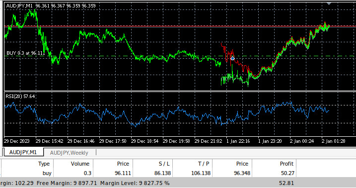
图10：我们交易历史数据的EA

结论

在本文中，我们阐述了为什么交易者预测价格变动可能比预测更高高点和更低低点更有利。希望读完本文后，您能够根据自己的风险承受能力和财务目标，更有信心地判断这一交易策略是否适合您。

线性判别分析（LDA）算法利用贝叶斯定理估算概率，并假设类内均值和共同方差的正态分布，来模拟每个类内输入变量的分布。LDA通过计算判别值来有效区分类别特征，这些判别值能够最大化类别间的分离度并最小化类内方差。然而，LDA的假设可能会限制其透明度和可解释性，且在没有进行广泛参数调整的情况下，其性能可能不如更简单的模型。我们在默认设置下对日数据进行的测试揭示了潜在的性能问题，这表明如果有更多数据和计算资源，可能会取得更好的结果。

虽然使用更大的数据集进行重复分析可能会提供更多见解，但这种方法只有在具备足够计算能力的情况下才可行。我们采用了10折时间序列交叉验证，这意味着每个模型都被训练了10次。随着数据集大小的增加，模型训练时间可能会呈指数级增长。