
Lorentzian Classification Open Source
- Индикаторы
- Версия: 1.0

The official MetaTrader 5 port of jdehorty's Lorentzian Classification indicator predicts the direction of future price movement from historical price data using Lorentzian distance.
Overview
A Lorentzian Distance Classifier (LDC) is a machine learning classification algorithm capable of categorizing historical data from a multi-dimensional feature space. This indicator demonstrates how Lorentzian Classification can be used to predict the direction of future price movements. Each bar is classified by price direction over a fixed 4-bar horizon using Lorentzian distance as the metric for distance-based classification.
The full source code is published on GitHub under the AI Edge (artificial-intelligence-edge) organization. This is the official AI Edge implementation for MetaTrader 5, derived from the same Lorentzian Classification algorithm originally authored for TradingView.
Background
In physics, Lorentzian space is perhaps best known for its role in describing the curvature of space-time in Einstein's theory of General Relativity (2). This abstract concept from theoretical physics also has tangible applications in the analysis of financial time-series data.
It has been hypothesized that Lorentzian space is well-suited for analyzing time-series data (4), (5). Several empirical studies support this: Lorentzian distance is more robust to outliers and noise than the commonly used Euclidean distance (1), (3), (6), and has been shown to outperform dozens of other distance metrics, including Manhattan distance, Bhattacharyya similarity, and Cosine similarity (1), (3). Across a wide variety of time-series datasets, the Lorentzian Distance metric consistently scores among the highest mean accuracy results (1).
Euclidean distance is commonly used as the default metric for pattern similarity measurement, but it may not be optimal for financial market data. Financial data can be significantly distorted by proximity to major events — FOMC meetings, central bank announcements, geopolitical shocks. This event-driven distortion can be framed as analogous to the gravitational warping that a massive object imposes on the space-time continuum. For financial markets, the analogous continuum is "price-time."
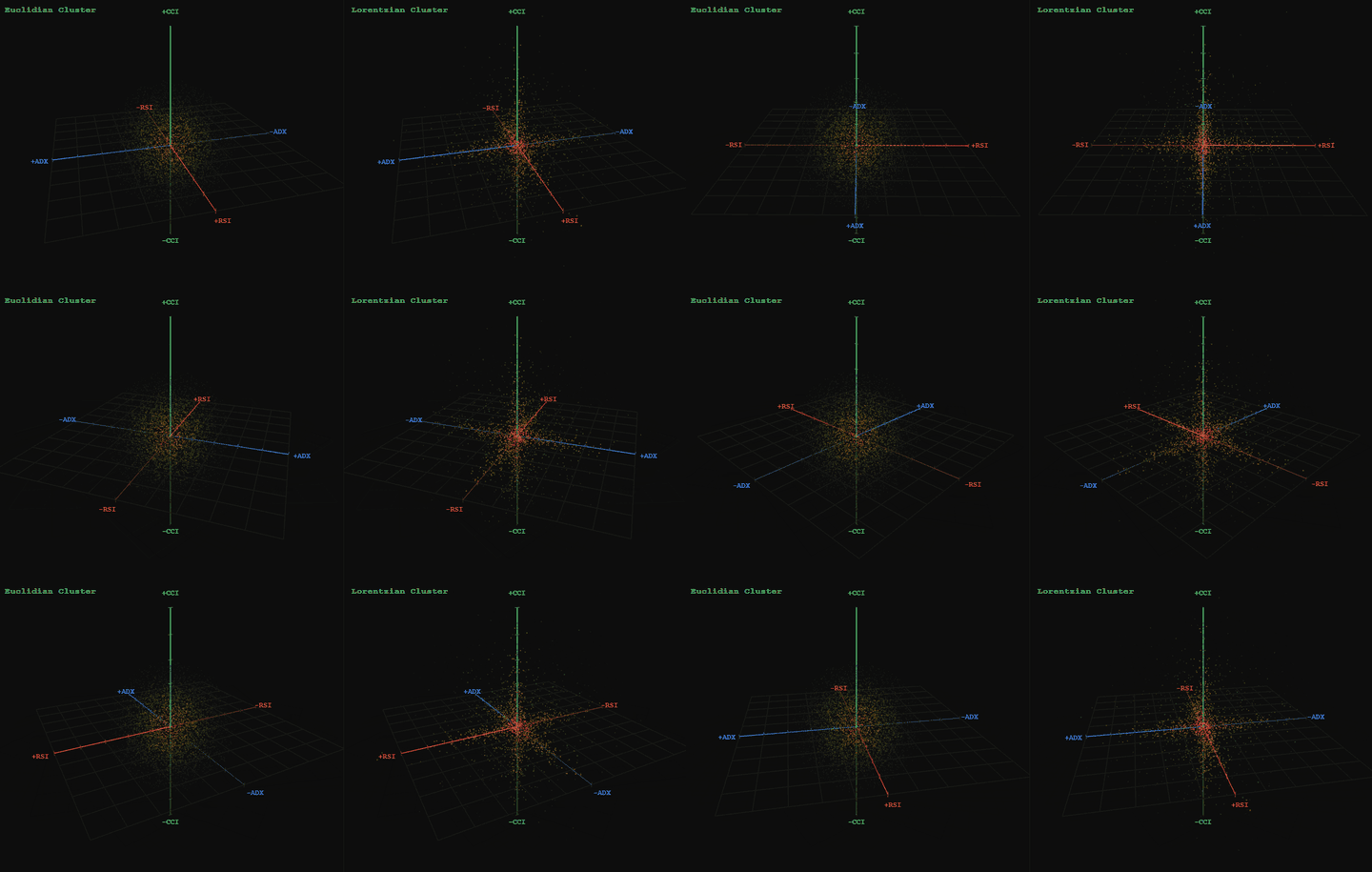
A side-by-side comparison of how neighborhoods of similar historical points appear in three-dimensional Euclidean space and Lorentzian space is included in the gallery (S1).
In that comparison, Lorentzian space better accommodates the warping of price-time because the Lorentzian distance function compresses the Euclidean neighborhood such that the new neighborhood distribution clusters around each of the major feature axes in addition to the origin itself. This means that even though some nearest neighbors are identical regardless of which metric is used, Lorentzian space also admits historical points that a Euclidean metric would never surface.
Intuitively, this makes sense. The price action that occurs in the hours after a central bank speech will resemble some of the previous times that same event occurred — regardless of whether the market was overbought or oversold, or whether macro conditions were broadly bullish or bearish. Euclidean distance misses these neighbors, often surfacing irrelevant data from the day before the event instead. Lorentzian distance accounts for the warping of price-time caused by the event and frees the model from the temporal bias imposed by the structure of a raw time series.
For implementation details of the classification algorithm, check out the source code.
How to Use
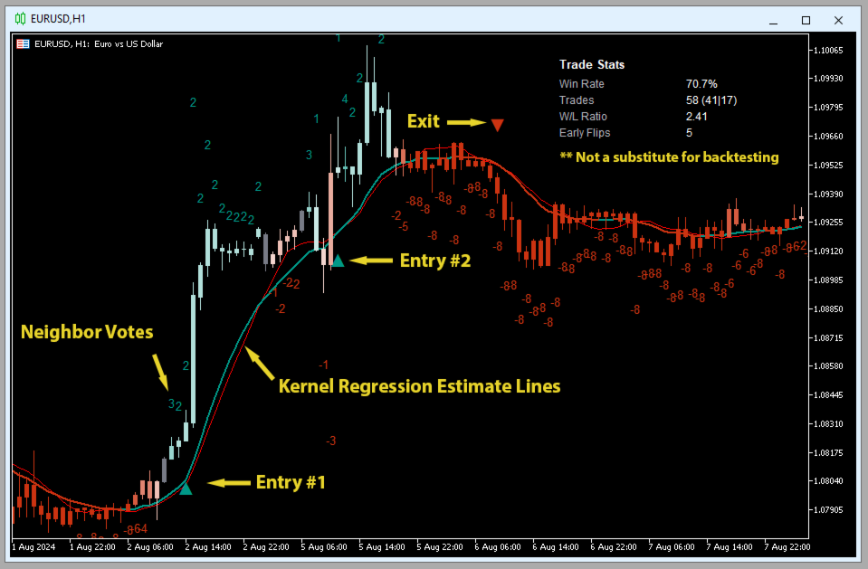
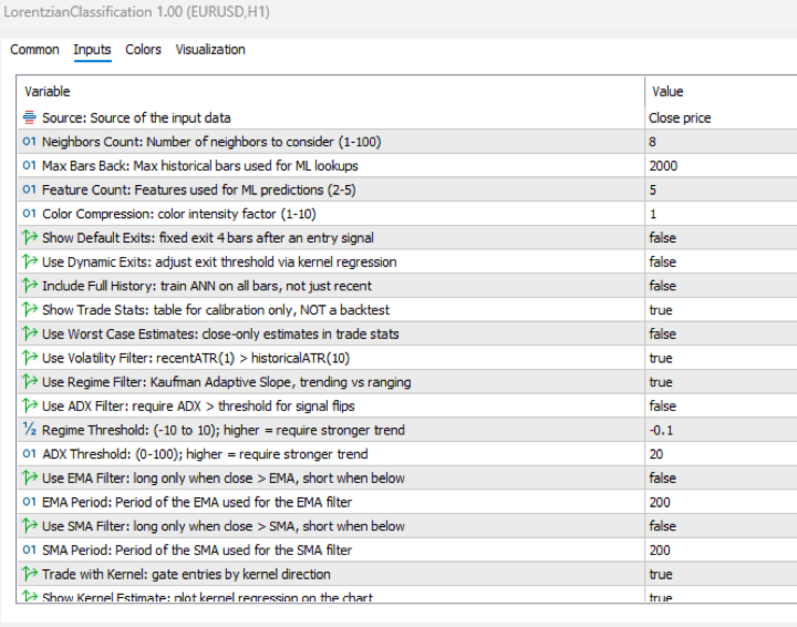
The indicator plots a color-coded bar overlay, two kernel regression estimate lines, and bullish/bearish signal labels directly on the chart. A trade stats table in the corner displays real-time win rate feedback for use in feature engineering. All visual elements and their controls, including the trade stats table, are shown in the gallery (S2, S3).
Reading the Signals
Each bar is assigned an integer prediction value by the model. More positive values correspond to more bullish sentiment, and more negative values correspond to more bearish sentiment — sequential patterns in these values can help identify fractals and distinguish potential inflection points from noise, rather than relying on any single bar's classification alone.
The kernel estimate lines are computed via kernel regression using a Rational Quadratic Kernel. It serves as additional confirmation of the model's bar-by-bar predictions.
Suggested exit points can be toggled on via the settings menu. Strict exits are based on the model's training interval (4 bars), while Dynamic Exits make suggestions based on real-time kernel regression.
The trade stats table is a real-time readout of trade performance for the selected number of historical bars (default 2000). It is not a robust backtesting method — by default it only reflects whether a historical trade was profitable 4 bars after entry, or, in Dynamic Exits mode, whether it was profitable after the Dynamic Exit was executed. It is intended to support real-time feature engineering, helping calibrate the model's settings to a given chart.
Early Flips, shown in the trade stats table, counts instances where a new ML signal was generated before the prior trade's exit was reached. A high count can indicate a choppy market and may suggest enabling additional signal filters.
General Settings
- Source — Default: "Close price". Controls the input data source.
- Neighbors Count — Default: 8, min: 1, max: 100. Controls the number of neighbors to consider.
- Max Bars Back — Default: 2000.
- Feature Count — Default: 5, min: 2, max: 5. Controls the number of features used for predictions.
- Color Compression — Default: 1, min: 1, max: 10. Controls the compression factor for the color scale intensity.
- Show Exits — Default: false. Shows exit arrow markers on the chart. Strict exits are based on the model's training interval (4 bars); see Use Dynamic Exits below for kernel-based exits.
- Use Dynamic Exits — Default: false. Controls whether to dynamically extend the exit threshold based on kernel regression, reducing premature exits.
- Include Full History — Default: false. When enabled, searches the full bar history for training; when disabled, uses only the most recent Max Bars Back bars.
- Show Trade Stats — Default: true. Controls whether to display the trade stats table (calibration only — not a backtest). By default reflects profitability 4 bars after entry, or at the Dynamic Exit if Use Dynamic Exits is enabled.
- Use Worst Case Estimate — Default: false. When enabled, uses bar close instead of mid-bar price for trade stats entries, producing a more conservative estimate consistent with traditional backtest results.
Filters Settings
- Use Volatility Filter — Default: true. Controls whether to apply the volatility filter.
- Use Regime Filter — Default: true. Controls whether to apply the trend detection filter.
- Use ADX Filter — Default: false. Controls whether to apply the ADX filter.
- Regime Threshold — Default: -0.1, min: -10, max: 10. Controls the Regime Detection filter for identifying trending vs. ranging conditions.
- ADX Threshold — Default: 20, min: 0, max: 100. Controls the ADX threshold for identifying trending vs. ranging conditions.
- Use EMA Filter — Default: false. When enabled, longs require close above the EMA and shorts require close below it.
- EMA Period — Default: 200. Period of the EMA used for the EMA filter.
- Use SMA Filter — Default: false. When enabled, longs require close above the SMA and shorts require close below it.
- SMA Period — Default: 200. Period of the SMA used for the SMA filter.
Kernel Regression Settings
- Trade with Kernel — Default: true. Controls whether to trade with the kernel.
- Show Kernel Estimate — Default: true. Controls whether to display the kernel estimate on the chart.
- Use Kernel Smoothing — Default: false. Crossover-based smoothing: fewer color flips, more ML entries.
- Lookback Window — Default: 8, min: 3. Controls the number of bars used for the estimation. Recommended range: 3–50.
- Relative Weighting — Default: 8. Controls the relative weighting of time frames. Recommended range: 0.25–25.
- Start Regression at Bar — Default: 25. Controls the bar index at which regression begins. Recommended range: 2–25.
- Kernel Lag — Default: 2. Lag used for crossover detection; lower values produce earlier crossovers. Recommended range: 1–2.
Feature Engineering Settings
Note: The Feature Engineering section is for fine-tuning the features used for predictions. The default values are optimized for the 4H to 12H timeframes for most charts but should work reasonably well across other timeframes.
There are five feature slots (Feature 1–5), each independently configurable. The Feature Count setting (from General Settings) controls how many feature slots will be used. For example, if Feature Count is 3 then Feature 1, Feature 2, and Feature 3 will be used. At least 2 features must be active. For each slot, you choose which feature type to use from the following four options — RSI, WT, CCI, and ADX. After choosing a type, set that slot's two parameters, Parameter A and Parameter B. What these parameters control depends on the type you chose for that slot:
- RSI — Parameter A: RSI period. Parameter B: EMA smoothing period applied to the RSI.
- WT (WaveTrend) — Parameter A: channel length. Parameter B: average length (second-stage smoothing).
- CCI — Parameter A: CCI period. Parameter B: EMA smoothing period applied to the CCI.
- ADX — Parameter A: ADX period. Parameter B: not used — ADX ignores it.
Using the same type in more than one slot (e.g. RSI in both Feature 1 and Feature 5) is allowed and counts as two separate features, typically with different parameter values.
Defaults by slot:
- Feature 1 — RSI. Parameter A (period): 14. Parameter B (smoothing): 1.
- Feature 2 — WT. Parameter A (channel length): 10. Parameter B (average length): 11.
- Feature 3 — CCI. Parameter A (period): 20. Parameter B (smoothing): 1.
- Feature 4 — ADX. Parameter A (period): 20. Parameter B: not used.
- Feature 5 — RSI. Parameter A (period): 9. Parameter B (smoothing): 1.
Display Settings
- Show Bar Colors — Default: true. Controls whether to show bar colors.
- Show Bar Prediction Values — Default: true. Controls whether to show the model's evaluation of each bar as an integer.
- Use ATR Offset — Default: false. Controls whether to use ATR-based offset instead of the bar prediction offset.
- Bar Prediction Offset — Default: 0, min: 0. Controls the offset of bar predictions as a percentage from the bar high/low.
Source Code
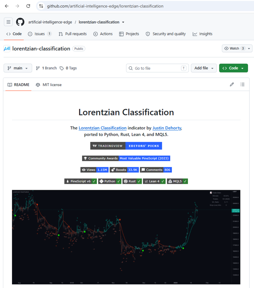
The complete MQL5 source code is published on GitHub under the AI Edge organization. The GitHub page is shown in the gallery (S4).
Risk Disclosure
Trading involves significant risk of loss. This indicator classifies historical market states and provides signals for evaluation by the trader. It does not guarantee profitable outcomes. Past classification performance does not predict future results.
Works Cited
- R. Giusti and G. E. A. P. A. Batista, "An Empirical Comparison of Dissimilarity Measures for Time Series Classification," 2013 Brazilian Conference on Intelligent Systems, Oct. 2013, DOI: 10.1109/bracis.2013.22.
- Y. Kerimbekov, H. S. Bilge, and H. H. Ugurlu, "The use of Lorentzian distance metric in classification problems," Pattern Recognition Letters, vol. 84, 170–176, Dec. 2016, DOI: 10.1016/j.patrec.2016.09.006.
- A. Bagnall, A. Bostrom, J. Large, and J. Lines, "The Great Time Series Classification Bake Off: An Experimental Evaluation of Recently Proposed Algorithms." ResearchGate, Feb. 04, 2016.
- H. S. Bilge, Yerzhan Kerimbekov, and Hasan Huseyin Ugurlu, "A new classification method by using Lorentzian distance metric," ResearchGate, Sep. 02, 2015.
- Y. Kerimbekov and H. Sakir Bilge, "Lorentzian Distance Classifier for Multiple Features," Proceedings of the 6th International Conference on Pattern Recognition Applications and Methods, 2017, DOI: 10.5220/0006197004930501.
- V. Surya Prasath et al., "Effects of Distance Measure Choice on KNN Classifier Performance - A Review." [Online].
Acknowledgements
Original indicator:
- veryfid — For many invaluable insights, discussions, and advice that helped shape this project.
- capissimo — For open-sourcing ideas regarding various nearest-neighbor implementations, several of which helped inspire the original undertaking.
- RikkiTavi — For many invaluable physics-related conversations and for help developing a mechanism for visualizing various distance algorithms in 3D using JavaScript.
- jlaurel — For invaluable literature recommendations that helped ground the underlying subject matter.
- annutara — For beta-testing the original indicator and sharing helpful ideas and insights early in its development.
- jasontaylor7 — For beta-testing the original indicator and many helpful conversations that shaped the backtesting workflow.
- meddymarkusvanhala — For beta-testing the original indicator.
- dlbnext — For detailed backtesting of the original indicator and for sharing ideas on improving the user experience.



































It will be good if there is buy and sell signal alerts