Working with ONNX Models in MQL5 (Part 3): Drawing the Neurons and the Weights Between Them
 330
 0

Introduction
In the previous part, we put the model on the chart and could finally see its shape. The layers sit in the right order, the branches read as branches, and clicking a weight tells us its range and its spread. What none of it shows is the network. A box marked "Gemm" with a row reading twenty-four by sixteen tells us a matrix is in there, and stops. The matrix holds which input reaches which neuron, whether each connection pushes or pulls, and which inputs dominate. None of that is drawn. We see the architecture, but the weights remain just numbers in a panel. This article is for MetaQuotes Language 5 (MQL5) developers and algorithmic traders who want to look inside a trained model rather than at its outline.
The way in is a detail worth stating plainly, because everything here follows from it. A dense layer's weight is a matrix, and that matrix is already the answer: the value at row sixteen, column three is the strength of the connection from the sixteenth input to the third neuron. In our previous article (Part 2), we parsed those numbers and left them sitting in a list. Now we draw them. We work out where each row of neurons sits, read each weight matrix as the connections joining two rows, and color every line by what it carries. We will cover the following topics:
- Understanding Dense Layers and Weight Matrices
- Building the Neuron Arrangement
- Drawing Neurons and Weighted Connections
- Switching Between the Graph and the Neurons
- Visualization
- Conclusion
By the end of this article, we will be able to:
- Read a weight matrix as a connection map between two rows of neurons, including the case where an operator stores it the other way round.
- Work out how many neurons a layer holds and where its row belongs, following the same value names that built the graph.
- Draw each stored connection colored by the sign and strength of the weight it carries, within the limits the view sets on stored values and lines.
- Decline to show the view with a specific reason when a model has no neuron pairs to draw, rather than inventing a picture.
Understanding Dense Layers and Weight Matrices
A dense layer does one thing: it multiplies what comes in by a matrix and adds a bias. The bias shifts each neuron on its own and is not part of any connection, so the matrix is where the connections live, and every number in it is one connection. Take a matrix of sixteen rows and twenty-four columns. Row three, column seven holds a single value, and that value is the strength with which the third incoming number reaches the seventh neuron. Positive, and it pushes that neuron up when the incoming value is positive. Negative, and it pulls it down. Near zero, and the two are barely joined at all.
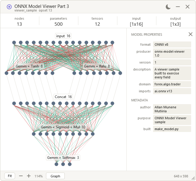
The weight is the strength of the link, not the size of the contribution, since the contribution is the weight multiplied by whatever value actually arrives on that input. A large weight on an input that is usually small moves the neuron less than the picture suggests. So we already have everything a picture needs: sixteen circles on one row, twenty-four on the next, and three hundred and eighty-four lines between them, each colored by the number sitting at its own position in the matrix. See an illustration below of the weight matrix as connections.
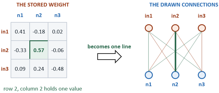
Some operators store that matrix with one row per incoming value, and others store it the other way round, with one row per neuron. For a non-square matrix, the shape often reveals the orientation. We can verify it against the neuron counts of adjacent layers. For a square matrix we cannot, and in either case the reliable signal is the attribute the exporter writes rather than the shape we infer. If we read a transposed matrix as non-transposed, the picture may still look plausible, but every neuron will connect to the wrong partner. Nothing errors, and nothing looks broken. So we read the "transB" attribute and index accordingly, treating the matrix as stored one row per incoming value unless that attribute is present and set.
This all works because a dense layer genuinely has one weight per pair of neurons. A convolution does not: its weights are a small filter slid across an input, so its connections are local and the same handful of numbers is shared at every position rather than one weight sitting at each pair. A recurrent layer packs several gates into one matrix, and an attention layer splits its weights across heads, so a single line drawn between two neurons misstates what those parameters hold. None of these layers are unconnected. They are connected differently, and a dense matrix drawing is the wrong display for them. Lines drawn anyway would look convincing, which is the danger, so where a model is not made of dense layers, we decline the view and say why. In a nutshell, here is an illustration of our objectives.
Building the Neuron Arrangement
The graph arrangement from the previous part places layers, and here we need something finer: rows of individual neurons and the connections between them. So we build a second arrangement alongside it, using the same value names for a different purpose.
//+------------------------------------------------------------------+
//| One row of neurons the view draws                                |
//+------------------------------------------------------------------+
struct OmvBand
  {
   // Count the neurons standing on this row
   int               count;
   // Name what produced the row and what was applied to it
   string            label;
   // Place the row across the arrangement
   int               x;
   // Place the row down the arrangement
   int               y;
   // Measure how wide the row of circles runs
   int               w;
   // Record how far the row sits from the graph input
   int               rank;
  };
First, we define the "OmvBand" structure to hold one row of neurons, keeping how many are on it, where it sits, and how far it lies from the graph input. Note that a row does not correspond to a layer. An activation changes the numbers on a row without changing how many there are, so it belongs to the row it modifies rather than opening one of its own, and the label is where we record that. Next, we describe what joins two rows together.
Describing a run of connections
Between two rows sits an entire weight matrix, so we record the pair once rather than every line separately.
//+------------------------------------------------------------------+
//| One run of connections between two rows                          |
//+------------------------------------------------------------------+
struct OmvWeb
  {
   // Name the row the connections leave
   int               from;
   // Name the row the connections arrive at
   int               to;
   // Index the tensor holding the weights, or a negative when structural
   int               tensor;
   // Offset the arriving row when several runs share it
   int               offset;
   // Mark a weight matrix the operator stores the other way round
   bool              transposed;
  };
Then, we define the "OmvWeb" structure to name the two rows and the tensor whose numbers join them. A negative tensor index marks a run carrying no weights, which is how we record a layer that merely joins two rows, and "offset" says where an arriving row lands when several runs share it. The "transposed" flag tells us which way round to read the matrix when we come to draw it. Before we can use either structure, we need to know which operators produce a row.
Sorting the operators
Not every layer creates neurons, and telling the two apart is what the whole walk rests on.
//+------------------------------------------------------------------+
//| Report whether an operator multiplies by a weight matrix         |
//+------------------------------------------------------------------+
bool COmvNeurons::IsDense(const string op) const
  {
//--- Only these two carry a two-dimensional weight between neuron rows
   return (op == "Gemm" || op == "MatMul");
  }

//+------------------------------------------------------------------+
//| Report whether an operator works on one value in place           |
//+------------------------------------------------------------------+
bool COmvNeurons::IsUnary(const string op) const
  {
//--- These change the values on a row without changing how many there are
   return (op == "Relu" || op == "Tanh" || op == "Sigmoid" || op == "Softmax" ||
           op == "LeakyRelu" || op == "Elu" || op == "Sqrt" || op == "Abs" ||
           op == "Cast" || op == "Identity" || op == "Clip" || op == "Erf");
  }
Here, we define "IsDense" to name the only two operators that carry a weight matrix between rows of neurons, and "IsUnary" to name those that reshape the numbers already on a row. We keep the lists explicit rather than clever, so an operator we have not thought about falls through to neither and is declined instead of being quietly assumed harmless. Two matching routines handle operators that pair a row with a constant and those that only rearrange it. With the sorting settled, we can open a row.
Opening a row
Every row the walk creates passes through one routine, so the bounds are checked in a single place.
//+------------------------------------------------------------------+
//| Open a new row of neurons                                        |
//+------------------------------------------------------------------+
int COmvNeurons::AddBand(const int count, const string label)
  {
//--- Decline a row beyond what the view may stack
   if(m_bands >= ON_MAX_BANDS || count <= 0)
      return -1;
//--- Describe the row
   OmvBand band;
   band.count = count;
   band.label = label;
   band.x = 0;
   band.y = 0;
   band.w = 0;
   band.rank = 0;
//--- Append it to the arrangement
   ArrayResize(m_band, m_bands + 1);
   m_band[m_bands++] = band;
   return m_bands - 1;
  }
Next, we define "AddBand" to append a row and return its index, declining anything past the stacking limit or with no neurons on it. A single entry point centralizes the checks. Callers can treat a negative return as a rejection and stop immediately. Every caller passes a positive count, the input row and the dense layers after checking it and the joining row as a sum of rows that already hold neurons, so a negative return always means the stacking limit was reached, which is the reason the caller reports. We leave the positions at zero here and settle them once the whole walk is done, and we know how deep it runs. Now we can walk the model.
Reading a dense layer
When we meet an operator that multiplies by a matrix, we open the row it produces and record the run joining it to the row before.
//+------------------------------------------------------------------+
//| Follow the value names into rows of neurons                      |
//+------------------------------------------------------------------+
bool COmvNeurons::Build(COmvModel &model)
  {
//--- Existing logic
      //--- A dense layer opens a row and connects to it through its weights
      if(IsDense(node.op) && feds > 0 && weight >= 0)
        {
         //--- Take whether the operator stores its weights the other way round
         bool flipped = false;
         for(int a = 0; a < node.attrCount; a++)
            if(node.attrName[a] == "transB" && node.attrValue[a] == "1")
               flipped = true;
         //--- Take both widths from whichever axes the storage implies
         OmvTensor w;
         model.TensorAt(weight, w);
         const int outWide = flipped ? w.dim[0] : w.dim[1];
         const int inWide = flipped ? w.dim[1] : w.dim[0];
         //--- Refuse a weight matrix with an empty axis
         if(outWide <= 0 || inWide <= 0)
           {
            m_reason = node.op + " carries a weight matrix with an empty axis";
            return false;
           }
         //--- Refuse a weight matrix whose input axis does not match the row feeding it
         if(inWide != m_band[fed[0]].count)
           {
            m_reason = node.op + " expects " + IntegerToString(inWide) + " inputs, but the row feeding it holds "
                       + IntegerToString(m_band[fed[0]].count);
            return false;
           }
         const int made = AddBand(outWide, node.op);
         if(made < 0)
           {
            m_reason = "the model has more layers than the view can stack";
            return false;
           }
         //--- Record the run of connections the weight describes
         OmvWeb web;
         web.from = fed[0];
         web.to = made;
         web.tensor = weight;
         web.offset = 0;
         web.transposed = flipped;
         ArrayResize(m_web, m_webs + 1);
         m_web[m_webs++] = web;
         //--- Stand the produced name on the new row
         if(node.emitCount > 0 && named < ArraySize(names))
           {
            names[named] = node.emits[0];
            bands[named] = made;
            named++;
           }
         continue;
        }
//--- Existing logic
Inside "Build", we read the attributes we parsed in the previous part, looking for the flag that says the matrix is stored the other way round. That flag decides how many neurons the new row holds, since the count comes from a different axis, and how we will index the matrix when we draw it. Before opening the row, we check that neither axis is empty and that the input axis matches the width of the row feeding the layer, and we refuse the view with a reason naming the layer when either check fails, so a mismatched matrix never draws as plausible lines.
We then record the run and store the produced value name on the new row, which is how the next layer reading that name finds its way here. A joining layer follows the same shape, opening a row as wide as everything arriving and recording one run per source with its own offset. With rows opening correctly, we handle the layers that open none.
Folding activations onto the row they change
An activation does not create neurons, so giving it a row of its own would double the picture with nothing between the copies.
//+------------------------------------------------------------------+
//| Follow the value names into rows of neurons                      |
//+------------------------------------------------------------------+
bool COmvNeurons::Build(COmvModel &model)
  {
//--- Existing logic
      //--- These change the numbers on a row without changing how many there are
      if((IsUnary(node.op) || IsBinary(node.op) || IsShape(node.op)) && feds > 0)
        {
         //--- Stand the produced name on the same row and note what was applied
         if(node.emitCount > 0 && named < ArraySize(names))
           {
            names[named] = node.emits[0];
            bands[named] = fed[0];
            named++;
           }
         if(IsUnary(node.op) || IsBinary(node.op))
            m_band[fed[0]].label += " + " + node.op;
         continue;
        }
      //--- A layer reading only stored tensors touches no row at all
      if(feds == 0)
         continue;
      //--- A dense layer whose weights are computed rather than stored
      if(IsDense(node.op))
        {
         m_reason = node.op + " takes its weights from another layer, not from a stored tensor";
         return false;
        }
//--- Existing logic
  }
Finally, we store the produced name on the row that fed it and append the operator to that row's label, so a row reads as "Gemm + Relu" rather than appearing twice. A layer reading only stored tensors touches no row at all and is skipped outright. The two rejections below keep the picture honest: a dense layer whose weights come from another layer rather than a stored tensor says exactly that rather than being lumped in with unsupported operators, and anything else we did not classify is declined by name. With every row opened and every run recorded, we can draw them.
Drawing Neurons and Weighted Connections
Every row is open, and every run is recorded, but nothing has a position yet. So we settle the depths, lay the rows out, and then draw one line per stored number in each matrix.
//+------------------------------------------------------------------+
//| Follow the value names into rows of neurons                      |
//+------------------------------------------------------------------+
bool COmvNeurons::Build(COmvModel &model)
  {
//--- Existing logic
//--- Take how deep each row sits by walking the runs until nothing moves
   for(int pass = 0; pass < m_bands; pass++)
     {
      //--- Push every target one step deeper than the source that feeds it
      bool moved = false;
      for(int i = 0; i < m_webs; i++)
        {
         //--- Deepen the target only when the source now sits deeper
         const int want = m_band[m_web[i].from].rank + 1;
         if(m_band[m_web[i].to].rank < want)
           {
            m_band[m_web[i].to].rank = want;
            moved = true;
           }
        }
      //--- Stop as soon as a whole pass changes nothing
      if(!moved)
         break;
     }
//--- Existing logic
  }
First, in the "Build" method, we settle every depth by sweeping the runs repeatedly, pushing each target row to sit one step below whatever feeds it, and stopping as soon as a whole pass changes nothing. This is the same rule that ranked the layer boxes in the previous part, applied now to rows of neurons. Two rows fed by the same source come out at the same depth, which is what we want, because they run at the same stage. Next, we turn those depths into positions.
Laying the rows across
Rows sharing a depth belong side by side, so we measure each depth before placing anything on it.
//+------------------------------------------------------------------+
//| Follow the value names into rows of neurons                      |
//+------------------------------------------------------------------+
bool COmvNeurons::Build(COmvModel &model)
  {
//--- Existing logic
//--- Measure every row and find how deep the arrangement runs
   int deepest = 0;
   for(int i = 0; i < m_bands; i++)
     {
      //--- Take the width the circles occupy on this row
      m_band[i].w = m_band[i].count * ON_DOT + (m_band[i].count - 1) * ON_DOT_GAP;
      if(m_band[i].rank > deepest)
         deepest = m_band[i].rank;
     }
//--- Lay every rank across, so rows sharing a depth sit side by side
   int widest = 0;
   for(int r = 0; r <= deepest; r++)
     {
      //--- Add the widths of every row at this depth
      int across = 0, seen = 0;
      for(int i = 0; i < m_bands; i++)
         if(m_band[i].rank == r)
           {
            across += m_band[i].w;
            seen++;
           }
      if(seen > 1)
         across += (seen - 1) * ON_RANK_GAP;
      if(across > widest)
         widest = across;
     }
//--- Existing logic
  }
Then, we measure how wide each row of circles runs and find the deepest rank in the arrangement. We walk the depths and add up the widths of every row sitting at each one, allowing a gap between them, and keep the widest result. That figure is what every rank is centered against, so a depth holding one row and a depth holding two both sit centered on the same axis rather than drifting left. With positions settled, we draw the model.
Drawing one line per weight
Here the matrix becomes the picture, and the flag we recorded earlier decides whether every line lands on the right pair.
//+------------------------------------------------------------------+
//| Draw the neurons and the weights joining them                    |
//+------------------------------------------------------------------+
void COmvPanel::DrawNeurons(void)
  {
//--- Existing logic
      //--- Fetch the weights this run draws
      OmvTensor w;
      m_model.TensorAt(web.tensor, w);
      //--- Scale the color and thickness against the largest weight held
      const double span = MathMax(MathAbs(w.minValue), MathAbs(w.maxValue));
      if(span <= 0.0 || w.kept <= 0)
         continue;
      //--- Thin the run when a full matrix would be more lines than we can draw
      const int lines = a.count * b.count;
      const double keep = (lines > ON_MAX_LINES) ? (double)ON_MAX_LINES / lines : 1.0;
      const double floor = (keep < 1.0) ? span * (1.0 - keep) : 0.0;
      //--- Draw one line per weight, from each source neuron to each target
      for(int r = 0; r < a.count; r++)
         for(int c = 0; c < b.count; c++)
           {
            //--- Take the weight joining this pair, whichever way it is stored
            const int at = web.transposed ? c * a.count + r : r * b.count + c;
            if(at >= w.kept)
               continue;
            const double v = w.val[at];
            //--- Drop the weakest connections when the run had to be thinned
            if(MathAbs(v) < floor)
               continue;
            //--- Fade the line by how strong the weight is against the largest
            const double strength = MathAbs(v) / span;
            const uint ink = (v >= 0.0) ? m_th.linkUp : m_th.linkDown;
            const uchar alpha = (uchar)(ON_ALPHA_MIN + ON_ALPHA_SPAN * strength);
//--- Existing logic
           }
Next, we walk through every pair of neurons and reach into the matrix for the number joining them. The index is where the transposed flag pays off, since a matrix stored the other way round needs the row and column swapped, and reading it wrongly would join every neuron to the wrong partner while still producing a picture that looks entirely reasonable. We take the largest absolute weight in the tensor as our scale, then color each line by the sign and fade it by the strength relative to that scale, so a weight near zero is barely visible and the strongest connections dominate. It is worth being precise about what that does and does not do. Weights are not changed. However, opacity is normalized to the largest weight in the tensor, so strengths are comparable only within a layer, not across layers.
Nor is every connection always drawn, since two budgets keep a large model from stalling the chart. When reading the model, each tensor keeps its first 4,096 values in storage order, so in a larger matrix, the connections stored past that point are missing whatever their strength. Separately, a run of more than 20,000 lines is thinned by strength: weights below a floor that rises with how far the run exceeds that budget are skipped, so the weakest connections go first. Layers with no usable weights are skipped. Line opacity runs from 40 for the faintest weight to 215 for the strongest, set by "ON_ALPHA_MIN" and "ON_ALPHA_SPAN", so a weak weight stays visible while the strongest stand out. The small sample model fits well inside both budgets, so every connection in it is drawn, but on a larger layer, the view is a partial plot rather than an exhaustive one.
Drawing the neurons themselves
The circles go over the connections, so a dense field of lines never obscures the rows.
//+------------------------------------------------------------------+
//| Draw the neurons and the weights joining them                    |
//+------------------------------------------------------------------+
void COmvPanel::DrawNeurons(void)
  {
//--- Existing logic
      //--- Fetch this row
      OmvBand band;
      m_cells.BandAt(i, band);
      //--- Place it against the current pan and zoom
      const double y = top + m_panY + band.y * m_zoom;
      const double x = left + m_panX + band.x * m_zoom;
      //--- Draw one filled circle per neuron
      for(int j = 0; j < band.count; j++)
         m_cv.DiscAA((int)(x + j * pitch + dot * 0.5), (int)(y + dot * 0.5),
                     (int)MathMax(1.0, dot * 0.5), m_th.cell);
      //--- Name the row over its own center, so two rows never collide
      m_cv.Font((int)MathMax(1.0, MathRound(8 * m_zoom)));
      const string caption = band.label + "  " + IntegerToString(band.count);
//--- Existing logic
  }
Here, we place each row against the current pan and zoom exactly as the graph view does, then draw a circle per neuron with "DiscAA" so the edges stay smooth at any scale. The caption sits over the row's own center rather than beside it, which is what stops two rows sharing a depth from printing their names on top of each other. Every row carries its label and its neuron count, so a row reads as "Gemm + Relu 24" and tells us both what it applies to and how wide it is.
Saying why there is nothing to draw
When the arrangement declined to build, an empty canvas would leave us guessing.
//+------------------------------------------------------------------+
//| Draw the neurons and the weights joining them                    |
//+------------------------------------------------------------------+
void COmvPanel::DrawNeurons(void)
  {
//--- Existing logic
//--- Say why the view is empty when the model cannot be drawn
   if(!m_cells.Ready())
     {
      //--- Print the reason in the middle of the area
      m_cv.Font(9);
      string why[];
      const int room = right - left - OP_PAD * 4;
      if(room > 0 && m_cv.WrapText("Neuron view unavailable: " + m_cells.Reason(),
                                   room, why, 1) > 0)
         m_cv.TxtM((left + right) / 2, (top + bottom) / 2, why[0], m_th.muted);
      m_cv.NoClip();
      return;
     }
//--- Existing logic
  }
Finally, we print the reason the arrangement gave us rather than showing a blank area, so a model built from convolutions says so and names the operator that stopped us. We bound the message to the width available and return immediately, since there is nothing behind it to draw. With the drawing settled, we need a way to reach it. We define that logic in the following section.
Switching Between the Graph and the Neurons
We build the neuron arrangement beside the graph one, and both now exist with no way to choose between them. So we add a control to the footer, wire it to the pointer, and make the view we are looking at drive everything that measures the arrangement.
//+------------------------------------------------------------------+
//| Measure whichever view is showing                                |
//+------------------------------------------------------------------+
   int               ViewWide(void)     const { return m_neuronView ? m_cells.Width()  : m_layout.Width(); }
   int               ViewHigh(void)     const { return m_neuronView ? m_cells.Height() : m_layout.Height(); }
   int               ScaledW(void)      const { return (int)(ViewWide() * m_zoom); }
   int               ScaledH(void)      const { return (int)(ViewHigh() * m_zoom); }
First, we route every measurement through "ViewWide" and "ViewHigh", which ask the flag and hand back the size of whichever arrangement is showing. We do this rather than teach each caller about both, because the fit, the pan clamp, and both scrollbars all measure the arrangement, and any one of them left reading the graph would let the neurons scroll off the edge. Changing two methods gives us the whole behavior. Next, we draw the control that flips the flag.
Drawing the switch
The control sits in the footer beside the zoom, naming the view it takes us to.
//+------------------------------------------------------------------+
//| Draw the control that swaps between the two views                |
//+------------------------------------------------------------------+
void COmvPanel::DrawViewSwitch(void)
  {
//--- Name the view the control would take us to
   const string label = m_neuronView ? "Graph" : "Neurons";
//--- Take whether the control can be used at all
   const bool live = m_neuronView || m_cells.Ready();
//--- Light the face while the pointer rests on a control that works
   const bool hot = (m_hover == OH_VIEW && live);
   m_cv.RoundFill(m_rView[0], m_rView[1], m_rView[2], m_rView[3], 4,
                  hot ? m_th.hoverFace : m_th.btnFace);
   m_cv.RoundStroke(m_rView[0], m_rView[1], m_rView[2], m_rView[3], 4, 1,
                    live ? m_th.btnEdge : m_th.divider);
//--- Name it, in the muted ink when the model cannot be drawn as neurons
   m_cv.Font(8);
   m_cv.TxtM(m_rView[0] + m_rView[2] / 2, m_rView[1] + m_rView[3] / 2,
             label, live ? m_th.text : m_th.divider);
  }
Then, we define "DrawViewSwitch" to name the view the control takes us to rather than the one we are on, so the button reads "Neurons" while we look at the graph. We work out whether it can be used at all, since a model with no dense layers has nothing to switch to, and draw it in muted ink when it cannot. We dim the control rather than hide it, because a button that vanishes leaves us wondering where it went, while a dim one invites a hover. Now we give that hover something to say.
Telling us why a control is dim
A disabled button explains nothing on its own, so the tooltip carries the reason the arrangement gave us.
//+------------------------------------------------------------------+
//| Describe whatever the pointer is resting on                      |
//+------------------------------------------------------------------+
string COmvPanel::TipFor(const int hit)
  {
//--- Existing logic
      case OH_FIT:
         return m_neuronView ? "Fit neurons" : "Fit graph";
      case OH_VIEW:
         //--- Say why the control cannot be used rather than leaving it silent
         if(!m_neuronView && !m_cells.Ready())
            return "Neuron view unavailable: " + m_cells.Reason();
         return m_neuronView ? "Back to the graph" : "Show the neurons";
//--- Existing logic
  }
Here, we hand back the reason the arrangement gave us when the control is dim, so hovering over a disabled button tells us the model uses an operator with no neuron pairs to draw instead of leaving us to guess. We also make the fit tooltip follow the view, since it fits whichever arrangement is showing, and reading "Fit graph" while looking at neurons would be wrong. Finally, we act on the click.
Flipping the view
Pressing the control swaps the flag and settles everything the old view left behind.
//+------------------------------------------------------------------+
//| Route a mouse event into the panel                               |
//+------------------------------------------------------------------+
void COmvPanel::OnEvent(const int id, const long &lparam, const double &dparam, const string &sparam)
  {
//--- Existing logic
      //--- Swap the view, but only where the other one can be drawn
      else if(act == OH_VIEW)
        {
         //--- Decline to leave the graph when the model has no neurons to show
         if(m_neuronView || m_cells.Ready())
           {
            m_neuronView = !m_neuronView;
            //--- The neuron view has nothing selectable, so drop what the graph chose
            m_selected = -1;
            m_pickKind = OP_PICK_NONE;
            m_hoverNode = -1;
            m_hoverRow = -1;
            m_hoverLink = -1;
            m_litName = "";
            //--- The two arrangements differ in size, so refit rather than keep the pan
            FitGraph();
            m_bgValid = false;
           }
        }
//--- Existing logic
  }
Finally, we flip the flag on a click, guarding it the same way the drawing does, so a dim control does nothing when pressed. We clear the selection and every hover index on the way through, because a node picked in the graph is not drawn in the neuron view, and leaving it set would have the footer naming a layer that is nowhere on screen. We refit rather than keep the pan, since the two arrangements differ in size and the offset that centered one would strand the other off the edge. With the switch working, we can look at what it draws in the next section.
Visualization
We compile the program, load it onto a chart with the model sitting in the terminal's Files folder, and press the footer control to switch from the graph to the neurons. We built it on MetaTrader 5 build 6230, and regenerating the model with "make_model.py" needs Python 3.13.12 with numpy 2.5.2 and onnx 1.22.0. The result is shown in the video below.
During testing, the neuron view opened on rows of circles laid out by depth, with every layer sitting below whatever fed it and two layers reading the same value drawn side by side rather than stacked. Between each pair of rows sat one line per weight. Green marked positive weights and red negative, weak weights drew faint and strong ones solid. This revealed the learned structure without reading raw numbers. Each row carried its own label and neuron count, naming both the operator and any activation folded onto it. Zoom and pan held the arrangement inside its area throughout, and the footer control returned us to the graph whenever we wanted the layer view back.
Conclusion
We have opened the layer boxes and drawn what is inside them. The arrangement follows the same value names that built the graph, opening a row of neurons wherever a dense layer produces one and folding activations onto the row they change rather than doubling the picture. Each weight matrix becomes the connections between two rows, one line per stored number within the view's budgets, colored by the sign and faded by the strength, with the transposed flag deciding which way round we read it so every line lands on the pair it belongs to.
Where a model has no neuron pairs to draw, we decline the view and name the operator that stopped us instead of inventing a diagram. Where we once saw a box telling us a matrix was somewhere inside it, we now see the matrix itself. In the next part, we will train a model on real market data and run it on live bars, lighting each neuron by what it fires. Stay tuned.
Attachments
| S/N | Name | Type | Description |
|---|---|---|---|
| 1 | make_model.py | Python script | Builds the sample classification network and saves it as model.onnx under MQL5\Files\ONNX Model Viewer Part 3\ |
| 2 | OMV Protobuf.mqh | Include file | Defines the wire type constants and the byte cursor that decodes variable-length integers, tags, text, nested blocks and fixed-width values |
| 3 | OMV Model.mqh | Include file | Defines the node, tensor and port structures, and implements the parser that reads the layers, their attributes, the shapes between them, and the weights themselves |
| 4 | OMV Canvas.mqh | Include file | Provides the drawing surface, holding the clip rectangle, the pixel blend, the smoothed lines, discs and rounded panels, and the cached text measurements |
| 5 | OMV Panel.mqh | Include file | Arranges the graph and the neurons, draws both views with every connection colored by the weight it carries, and answers the mouse for hover, drag, zoom, selection and the view switch |
| 6 | ONNX Model Viewer Part 3.mq5 | Expert Advisor | The main program entry point that declares the model path, includes the four module headers, builds the panel on initialization, and forwards every chart event to it |
| 7 | MQL5.zip | Archive | A ready-to-extract archive with the MQL5 folder as its root. Unzip it into your MetaTrader 5 terminal data folder; every file is placed in its correct location, the code under MQL5\Experts\ONNX Model Viewer Part 3\ and the Python script under MQL5\Files\ONNX Model Viewer Part 3, ready to compile. |
The project is supported in Algo Forge: https://forge.mql5.io/29210372/Article-24337-Working-With-ONNX-Models-In-MQL5-Part-3
Warning: All rights to these materials are reserved by MetaQuotes Ltd. Copying or reprinting of these materials in whole or in part is prohibited.
This article was written by a user of the site and reflects their personal views. MetaQuotes Ltd is not responsible for the accuracy of the information presented, nor for any consequences resulting from the use of the solutions, strategies or recommendations described.