
Создание самооптимизирующихся советников на MQL5 (Часть 15): Идентификация линейных систем

Торговые системы представляют собой сложные приложения, которые должны работать в хаотичных и динамичных условиях — это сложная задача даже для самых опытных разработчиков. Невозможно заранее описать все корректные действия торговой системы, которые должно совершать торговое приложение, поскольку возможные рыночные исходы практически бесконечны. Сохранение контроля и обеспечение стабильной прибыльности в условиях такой неопределённости остаётся одной из самых сложных задач в алгоритмической торговле.
Простые стратегии могут казаться надежными в условиях стабильного рынка, однако как простые, так и сложные системы часто дают сбой при росте волатильности. Несмотря на это, такие области, как теория управления и обработка сигналов, по-видимому, используются недостаточно широко при решении этих задач. Теория управления, посвященная обеспечению устойчивости динамических и неопределенных систем, тесно связана с проблемами, с которыми ежедневно сталкивается наше сообщество алгоритмических трейдеров.
Классическая теория управления предполагает понимание системы на основе фундаментальных принципов — наличие явных формул, описывающих взаимосвязь между входными и выходными сигналами. Современные финансовые рынки, однако, не поддаются столь четкой математической структуре. Это привело к росту интереса к интеграции теории управления с машинным обучением, которое позволяет аппроксимировать эти зависимости непосредственно на основе данных, а не опираться на явные уравнения.
Этот подход имеет большой потенциал: даже не зная точных уравнений управления, специалисты-практики все равно могут научиться регулировать поведение системы на основе данных. Теория управления и алгоритмическая торговля преследуют одну и ту же цель — управление неопределённостью при одновременном обеспечении стабильности. Контроллер обратной связи не прогнозирует цены; он регулирует реакции системы, подавляя чрезмерные реакции на помехи и обеспечивая стабильную работу.
Системы управления обратной связью также повышают эффективность использования капитала, анализируя, в каких случаях капитал используется эффективно, и сокращая количество ненужных торговых операций. В сочетании с машинным обучением эти системы обретают способность самостоятельно адаптироваться, что повышает их точность, управляемость и надежность. Несмотря на очевидное пересечение, между теорией управления и алгоритмической торговлей по-прежнему существует значительный пробел в исследованиях — пробел, таящий в себе огромный потенциал.
В этой статье мы покажем, как теория управления может вдохнуть новую жизнь даже в самые простые торговые системы. Используя простую стратегию скользящего среднего — покупку при прорыве цены выше среднего значения и продажу при падении ниже него — мы изучаем, как контроллер обратной связи может вернуть стабильность и прибыльность стратегии, которую часто считают устаревшей. Хотя многие утверждают, что такие методы не работают, поскольку они «слишком хорошо известны», подобные аргументы не подкреплены эмпирическими данными. Вместо этого в нашем подходе используется контроллер обратной связи, который позволяет определить, когда и почему стратегия приносит успех или терпит неудачу.
Для нашего эксперимента мы реализовали классическую стратегию скользящего среднего и зафиксировали все параметры. Используя данные за два года (январь 2023 г. – май 2025 г.), мы оптимизировали период скользящего среднего в первой половине периода и проверили эффективность во второй, установив таким образом бенчмарк для сравнения. После того как этот базовый эталон был установлен, алгоритм управления с обратной связью обучался исключительно на основе поведения системы во время тестирования на исторических данных, без какой-либо настройки параметров.
Вначале как управляемая, так и неуправляемая системы работали одинаково, поскольку контроллер все еще находился в режиме наблюдения. Когда контроллер активировался, система с обратной связью показала заметное улучшение результатов.
- Общий убыток сократился с –575 до –333 долларов (сокращение неэффективного использования капитала на 42 %)
- Чистая прибыль выросла с –49 до +57 долларов
- Количество сделок сократилось с 78 до 51 (рост эффективности на 34 %).
- Доля прибыльных сделок выросла с 44% до 53%
- Коэффициент прибыльности — от 0,91 до 1,17, что означает рост рентабельности на 28 %.
Эти результаты, полученные при одинаковых рыночных условиях и системных ограничениях, демонстрируют стабилизирующий эффект управления с обратной связью. Там, где человеческая интуиция и традиционное моделирование достигают своих пределов, теория управления предлагает обоснованный путь вперед, раскрывая более глубокие взаимосвязи и нереализованный потенциал стратегий, которые давно считались исчерпанными.
Начало работы с MQL5
Чтобы приступить к разработке нашего приложения, сначала определим ключевые системные константы, которые остаются неизменными на протяжении всех упражнений. В последующих версиях количество констант будет увеличиваться, но мы планируем сохранять их из одной версии в другую.//+------------------------------------------------------------------+ //| Feedback Control Benchmark .mq5 | //| Copyright 2025, MetaQuotes Ltd. | //| https://www.mql5.com | //+------------------------------------------------------------------+ #property copyright "Copyright 2025, MetaQuotes Ltd." #property link "https://www.mql5.com" #property version "1.00" //+------------------------------------------------------------------+ //| System constants | //+------------------------------------------------------------------+ #define SYMBOL Symbol() #define MA_SHIFT 0 #define MA_MODE MODE_EMA #define MA_APPLIED_PRICE PRICE_CLOSE #define SYSTEM_TIME_FRAME PERIOD_D1 #define MIN_VOLUME SymbolInfoDouble(SYMBOL,SYMBOL_VOLUME_MIN)
Читателю следует иметь в виду, что цель данной базовой версии заключается в том, чтобы обеспечить благоприятный стартовый период для наших технических индикаторов. Поэтому мы задаем в качестве входных данных параметр настройки, который планируем впоследствии оптимизировать с помощью генетического алгоритма.
//+------------------------------------------------------------------+ //| Tuning parameters | //+------------------------------------------------------------------+ input group "Technical Indicators" input int MA_PERIOD = 10;//Moving average period
Далее мы загружаем библиотеки, необходимые для этого упражнения. Библиотеки Trade вполне достаточно.
//+------------------------------------------------------------------+ //| Libraries | //+------------------------------------------------------------------+ #include <Trade\Trade.mqh> CTrade Trade;
Мы также определяем важные глобальные переменные, такие как буферы для индикаторов «Скользящее среднее» и «Средний истинный диапазон» (ATR). ATR определяет наши уровни стоп-лосса и риска, которые остаются неизменными во всех упражнениях. Мы также добавляем глобальные переменные для отслеживания рыночных цен (открытие, максимум, минимум, закрытие) и дескрипторы для наших технических индикаторов.
//+------------------------------------------------------------------+ //| Global variables | //+------------------------------------------------------------------+ double ma[],atr[]; double ask,bid,open,high,low,close,padding; int ma_handler,atr_handler;
При первом запуске приложения мы инициализируем обработчики для индикаторов — один для скользящей средней и один для ATR. Индикатор ATR измеряет волатильность рынка и на основе полученных данных устанавливает уровни стоп-лосса и тейк-профита.
//+------------------------------------------------------------------+ //| Expert initialization function | //+------------------------------------------------------------------+ int OnInit() { //--- Initialize the indicator ma_handler = iMA(SYMBOL,SYSTEM_TIME_FRAME,MA_PERIOD,MA_SHIFT,MA_MODE,MA_APPLIED_PRICE); atr_handler = iATR(SYMBOL,SYSTEM_TIME_FRAME,14); return(INIT_SUCCEEDED); }
После закрытия приложения мы деинициализируем индикаторы и освобождаем занятые ими ресурсы в соответствии с рекомендациями по программированию на MQL5.
//+------------------------------------------------------------------+ //| Expert deinitialization function | //+------------------------------------------------------------------+ void OnDeinit(const int reason) { //--- Release the indicator IndicatorRelease(ma_handler); IndicatorRelease(atr_handler); }
Как только терминал получает новые данные о ценах, мы запускаем нашу торговую стратегию. Сначала мы проверяем, появление новой дневной свечи. В таком случае мы открываем не более одной сделки в день.
Наша торговая стратегия основана на сравнении ценовых уровней со скользящей средней. Однако при тестировании на исторических данных в MetaTrader 5 первая дневная свеча формируется в полночь, когда ценовые значения часто остаются неизменными и являются недостоверными. Чтобы этого избежать, наш алгоритм учитывает значения свечей и индикаторов за предыдущий день. По сути, приложение определяет сегодняшние действия на основе того, что произошло вчера.
Затем мы реализуем торговую стратегию, проверяя, находится ли цена закрытия выше или ниже скользящей средней, чтобы принять решение о покупке или продаже.
//+------------------------------------------------------------------+ //| Expert tick function | //+------------------------------------------------------------------+ void OnTick() { //--- Check if a new candle has formed datetime current_time = iTime(Symbol(),SYSTEM_TIME_FRAME,0); static datetime time_stamp; if(current_time != time_stamp) { //--- Update the time time_stamp = current_time; //--- If we have no open positions if(PositionsTotal()==0) { //--- Update indicator buffers CopyBuffer(ma_handler,0,1,1,ma); CopyBuffer(atr_handler,0,0,1,atr); padding = atr[0] * 2; //--- Fetch current market prices ask = SymbolInfoDouble(SYMBOL,SYMBOL_ASK); bid = SymbolInfoDouble(SYMBOL,SYMBOL_BID); close = iClose(SYMBOL,SYSTEM_TIME_FRAME,0); //--- Check trading signal if(close > ma[0]) Trade.Buy(MIN_VOLUME,SYMBOL,ask,ask-padding,ask+padding); if(close < ma[0]) Trade.Sell(MIN_VOLUME,SYMBOL,bid,ask+padding,ask-padding); } } } //+------------------------------------------------------------------+
После завершения выполнения мы отменяем определение всех ранее определённых системных констант.
//+------------------------------------------------------------------+ //| Undefine system constants | //+------------------------------------------------------------------+ #undef SYMBOL #undef SYSTEM_TIME_FRAME #undef MA_APPLIED_PRICE #undef MA_MODE #undef MA_SHIFT #undef MIN_VOLUME //+------------------------------------------------------------------+
В результате все это вместе составляет эталонную версию приложения.
//+------------------------------------------------------------------+ //| Feedback Control Benchmark .mq5 | //| Copyright 2025, MetaQuotes Ltd. | //| https://www.mql5.com | //+------------------------------------------------------------------+ #property copyright "Copyright 2025, MetaQuotes Ltd." #property link "https://www.mql5.com" #property version "1.00" //+------------------------------------------------------------------+ //| System constants | //+------------------------------------------------------------------+ #define SYMBOL Symbol() #define MA_SHIFT 0 #define MA_MODE MODE_EMA #define MA_APPLIED_PRICE PRICE_CLOSE #define SYSTEM_TIME_FRAME PERIOD_D1 #define MIN_VOLUME SymbolInfoDouble(SYMBOL,SYMBOL_VOLUME_MIN) //+------------------------------------------------------------------+ //| Tuning parameters | //+------------------------------------------------------------------+ input group "Technical Indicators" input int MA_PERIOD = 10;//Moving average period //+------------------------------------------------------------------+ //| Libraries | //+------------------------------------------------------------------+ #include <Trade\Trade.mqh> CTrade Trade; //+------------------------------------------------------------------+ //| Global variables | //+------------------------------------------------------------------+ double ma[],atr[]; double ask,bid,open,high,low,close,padding; int ma_handler,atr_handler; //+------------------------------------------------------------------+ //| Expert initialization function | //+------------------------------------------------------------------+ int OnInit() { //--- Initialize the indicator ma_handler = iMA(SYMBOL,SYSTEM_TIME_FRAME,MA_PERIOD,MA_SHIFT,MA_MODE,MA_APPLIED_PRICE); atr_handler = iATR(SYMBOL,SYSTEM_TIME_FRAME,14); return(INIT_SUCCEEDED); } //+------------------------------------------------------------------+ //| Expert deinitialization function | //+------------------------------------------------------------------+ void OnDeinit(const int reason) { //--- Release the indicator IndicatorRelease(ma_handler); IndicatorRelease(atr_handler); } //+------------------------------------------------------------------+ //| Expert tick function | //+------------------------------------------------------------------+ void OnTick() { //--- Check if a new candle has formed datetime current_time = iTime(Symbol(),SYSTEM_TIME_FRAME,0); static datetime time_stamp; if(current_time != time_stamp) { //--- Update the time time_stamp = current_time; //--- If we have no open positions if(PositionsTotal()==0) { //--- Update indicator buffers CopyBuffer(ma_handler,0,1,1,ma); CopyBuffer(atr_handler,0,0,1,atr); padding = atr[0] * 2; //--- Fetch current market prices ask = SymbolInfoDouble(SYMBOL,SYMBOL_ASK); bid = SymbolInfoDouble(SYMBOL,SYMBOL_BID); close = iClose(SYMBOL,SYSTEM_TIME_FRAME,0); //--- Check trading signal if(close > ma[0]) Trade.Buy(MIN_VOLUME,SYMBOL,ask,ask-padding,ask+padding); if(close < ma[0]) Trade.Sell(MIN_VOLUME,SYMBOL,bid,ask+padding,ask-padding); } } } //+------------------------------------------------------------------+ //+------------------------------------------------------------------+ //| Undefine system constants | //+------------------------------------------------------------------+ #undef SYMBOL #undef SYSTEM_TIME_FRAME #undef MA_APPLIED_PRICE #undef MA_MODE #undef MA_SHIFT #undef MIN_VOLUME //+------------------------------------------------------------------+
Определение благоприятных исходных условий
Теперь мы можем выбрать тестовую торговую стратегию и указать исторические даты для тестирования на исторических данных. В данном упражнении мы используем данные за период с 2023 по 2025 год, а также проводим тестирование на будущем периоде. Для тех читателей, кто не знаком с этим термином, поясним, что перспективное тестирование заключается в разделении периода бэктеста на сегменты, которые могут быть как равными по длине, так и разными. Здесь мы разделили набор данных пополам, установив значение параметра forward равным ½. Это позволяет генетическому оптимизатору настраивать параметры. Первая половина данных используется для настройки, вторая — для проверки (out-of-sample). Вторая половина набора данных скрыта от модели и используется в качестве набора для итоговой оценки; она раскрывается оптимизатору только после завершения обучения.
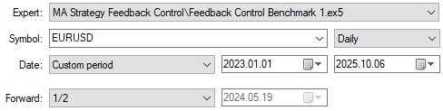
Рисунок 1: Выбор дней для бэк-тестирования в рамках нашей процедуры оптимизации
Теперь, когда мы понимаем важность перспективного тестирования, мы можем определить условия моделирования, в которых будет проводиться оценка нашей стратегии. Из-за ограничений сети я использовал режим моделирования «каждый тик» вместо режима «каждый тик на основе реальных тиков», хотя последний дает более реалистичные результаты и рекомендуется тем, у кого стабильное подключение. В целях оптимизации мы использовали быстрый генетический алгоритм для повышения эффективности; для более тщательного поиска можно использовать более медленную, полную версию. Входные параметры были определены с помощью их минимального и максимального значений, а также шага, чтобы ограничить диапазон работы оптимизатора.
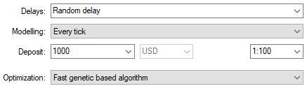
Рисунок 2: Выберите быстрый генетический алгоритм, который поможет нам определить подходящие начальные периоды индикаторов
Для начала мы установили параметр задержки на значение «случайная задержка», чтобы смоделировать реальную задержку на рынке.
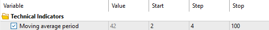
Рисунок 3: Параметры настройки нашего торгового приложения просты и понятны
Результаты бэктестинга оказались неудовлетворительными — ни одна из конфигураций не принесла прибыли.
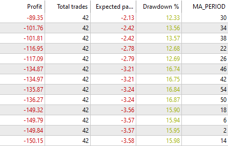
Рисунок 4: Результаты бэктеста выглядят нестабильными и требуют доработки
Точечные диаграммы подтвердили стабильные потери во всех испытаниях.
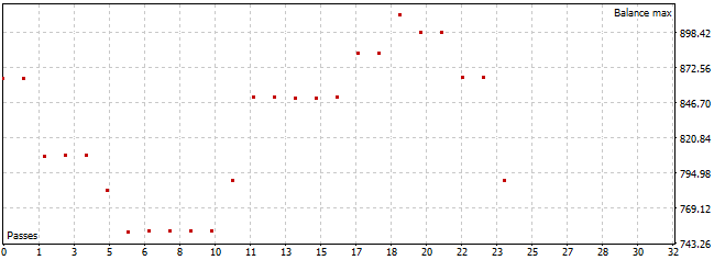
Рисунок 5: Судя по всему, ни одна из протестированных нами конфигураций не оказалась прибыльной в первой половине процесса оптимизации
Удивительно, но в тесте на будущие данные стратегия стала прибыльной, особенно при значении периода, равном 42. Хотя выбор наиболее эффективного результата сопряжён с риском переобучения, длительные периоды оценки снижают эту вероятность.
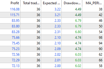
Рисунок 6: Результаты форвардного тестирования оказались более успешными, чем результаты бэк-тестирования, которые мы получили.
В ходе форвардного тестирования было выявлено множество наиболее прибыльных конфигураций, что свидетельствует о том, что стратегия может демонстрировать хорошие результаты при определенных условиях, но в своей нынешней форме может оказаться ненадежной. Надежная стратегия должна демонстрировать стабильные результаты на протяжении длительного времени, чего наша стратегия не сделала.
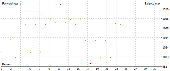
Рисунок 7: Результаты стратегии на данных, не участвовавших в обучении.
Определение наших эталонов
Чтобы определить контрольный уровень доходности, сначала выбираем скомпилированное приложение в нашей IDE, а затем указываем даты бэктеста — тот же период, который использовался ранее и который впоследствии применялся для форвард-тестирования.
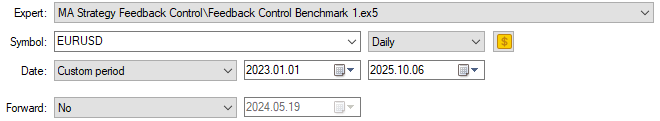
Рисунок 8: Проведение полного исторического бэктеста нашего торгового приложения с использованием оптимального периода, который мы определили
В ходе полного бэктеста с использованием 42-периодного параметра стратегия понесла общий убыток в размере 559 долларов по итогам 78 сделок, при этом коэффициент прибыльности составил 0,97, что свидетельствует о сокращении капитала в долгосрочной перспективе, а не о его росте.
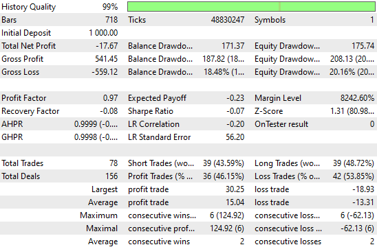
Рисунок 9: Анализ подробных статистических показателей нашего контрольного теста на исторических данных
Кривая капитала, полученная в результате применения этой версии нашей торговой стратегии, характеризуется высокой волатильностью, при этом в целом стратегия демонстрирует низкую эффективность. Даже в ходе первоначального бэктеста, целью которого было продемонстрировать лучшие результаты, полученные с помощью генетического оптимизатора, стратегия едва достигла безубыточности после двух лет торговли.
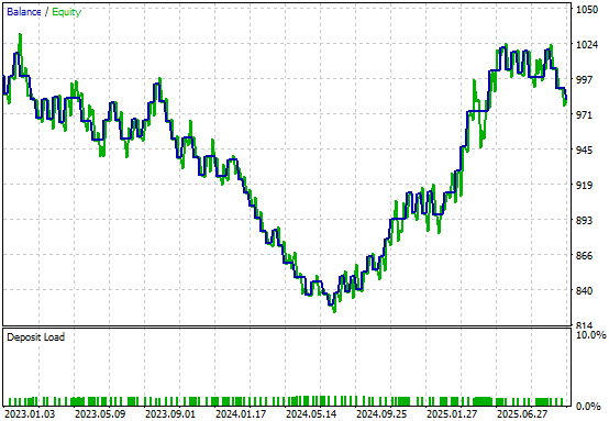
Рисунок 10: Кривая капитала, построенная на основе контрольной конфигурации нашего торгового приложения, выглядит весьма нестабильной
Улучшение наших первоначальных результатов
Теперь мы готовы приступить к повышению наших контрольных показателей рентабельности. Для начала мы определим дополнительные системные константы, расширив те, которые были введены ранее. Эти новые константы определяют параметры, необходимые для нашей модели — например, сколько данных о наблюдениях должен собрать регулятор с обратной связью, прежде чем скорректировать поведение стратегии.//+------------------------------------------------------------------+ //| System constants | //+------------------------------------------------------------------+ #define SYMBOL Symbol() #define MA_PERIOD 42 #define MA_SHIFT 0 #define MA_MODE MODE_EMA #define MA_APPLIED_PRICE PRICE_CLOSE #define SYSTEM_TIME_FRAME PERIOD_D1 #define MIN_VOLUME SymbolInfoDouble(SYMBOL,SYMBOL_VOLUME_MIN) #define OBSERVATIONS 90 #define FEATURES 7 #define MODEL_INPUTS 8
Мы также определяем новые глобальные переменные для хранения прогнозов, полученных с помощью нашей линейной системы, а также входных данных, целевых значений и матрицы исторических наблюдений.
//+------------------------------------------------------------------+
//| Global variables                                                 |
//+------------------------------------------------------------------+
double ma[],atr[];
double ask,bid,open,high,low,close,padding;
int    ma_handler,atr_handler,scenes;
bool   forecast;
matrix snapshots,b,X,y,U,S,VT,current_forecast;
vector s;
Функция инициализации советника была слегка изменена для подготовки этих глобальных переменных.
//+------------------------------------------------------------------+
//| Expert initialization function                                   |
//+------------------------------------------------------------------+
int OnInit()
  {
//--- Initialize the indicator
   ma_handler = iMA(SYMBOL,SYSTEM_TIME_FRAME,MA_PERIOD,MA_SHIFT,MA_MODE,MA_APPLIED_PRICE);
   atr_handler = iATR(SYMBOL,SYSTEM_TIME_FRAME,14);

//--- Prepare global variables
   forecast = false;
   snapshots = matrix::Zeros(FEATURES,OBSERVATIONS);
   scenes = -1;
   return(INIT_SUCCEEDED);
  }
При обновлении цен наша торговая логика проверяет, требуется ли прогноз, полученный с помощью линейной системы. Если система продолжает собирать данные, она пропускает этап прогнозирования и выполняет сделки в соответствии с прежней логикой. Как только будет собрано достаточное количество данных, запускается процесс прогнозирования. Независимо от открытых позиций система фиксирует периодические срезы данных при появлении каждой новой свечи, фиксируя состояние модели во времени.
Если позиции открыты, запускается метод прогнозирования по модели для получения линейного прогноза, который впоследствии может помочь определить время выхода из позиции. На данный момент наша цель состоит лишь в том, чтобы понаблюдать, способна ли эта линейная система с обратной связью регулировать поведение стратегии.
//+------------------------------------------------------------------+
//| Expert tick function                                             |
//+------------------------------------------------------------------+
void OnTick()
  {
//--- Check if a new candle has formed
   datetime current_time = iTime(Symbol(),SYSTEM_TIME_FRAME,0);
   static datetime time_stamp;

   if(current_time != time_stamp)
     {
      //--- Update the time
      time_stamp = current_time;
      scenes = scenes+1;

      //--- Check how many scenes have elapsed
      if(scenes == (OBSERVATIONS-1))
        {
         forecast   = true;
        }

      //--- If we have no open positions
      if(PositionsTotal()==0)
        {
         //--- Update indicator buffers
         CopyBuffer(ma_handler,0,1,1,ma);
                     CopyBuffer(atr_handler,0,0,1,atr);
            padding = atr[0] * 2;

         //--- Fetch current market prices
         ask = SymbolInfoDouble(SYMBOL,SYMBOL_ASK);
         bid = SymbolInfoDouble(SYMBOL,SYMBOL_BID);
         close = iClose(SYMBOL,SYSTEM_TIME_FRAME,1);

         //--- Do we need to forecast?
         if(!forecast)
           {
            //--- Check trading signal
            check_signal();
           }

         //--- We need a forecast
         else
            if(forecast)
              {
               model_forecast();
              }
        }

      //--- Take a snapshot
      if(!forecast)
         take_snapshot();

      //--- Otherwise, we have positions open
      else
        {
         //--- Let the model decide if we should close or hold our position
         if(forecast)
            model_forecast();

         //--- Otherwise record all observations on the performance of the application
         else
            if(!forecast)
               take_snapshot();
        }
     }
  }
//+------------------------------------------------------------------+
Логика торговли была переработана и вынесена в отдельный метод CheckSignal, который действует по тем же правилам: если открытых позиций нет, то покупать, когда цена выше скользящей средней, и продавать, когда ниже.
//+------------------------------------------------------------------+
//| Check for our trading signal                                     |
//+------------------------------------------------------------------+
void check_signal(void)
  {
   if(PositionsTotal() == 0)
     {
      if(close > ma[0])
        {
         Trade.Buy(MIN_VOLUME,SYMBOL,ask,ask-padding,ask+padding);
        }

      if(close < ma[0])
        {
         Trade.Sell(MIN_VOLUME,SYMBOL,bid,ask+padding,ask-padding);
        }
     }
  }
Составление прогноза предполагает подготовку и обновление снимков состояния. Сначала мы копируем существующие снимки, а затем обновляем их с помощью take_snapshots(). Затем подготавливаются входные данные (X) и целевое значение (y) нашей линейной системы: первая строка матрицы X представляет собой вектор, состоящий из единиц (пересечение с осью), а остальные строки содержат наблюдаемые значения системы. Цель — баланс счета на один шаг впереди снимков состояния.
Затем мы проводим сингулярное разложение (SVD) — алгоритм без учителя, который разлагает матрицу на ряд компонентов ранга 1, выявляя доминирующие корреляционные структуры в данных. Алгоритм возвращает один вектор и две матрицы, которые мы используем для построения нашей линейной системы. Вектор преобразуется в диагональную матрицу с помощью метода Diag(), после чего мы проверяем её ранг. Если значение отлично от нуля, мы вычисляем псевдообратную матрицу для оценки коэффициентов системы, которые хранятся в массиве b.
Далее мы извлекаем текущие рыночные данные и умножаем их на b, чтобы получить оценку по нашей линейной системе. Если прогнозируемый баланс превышает текущий, система приступает к торговле; в противном случае она ожидает более благоприятных рыночных условий. Заключительная проверка позволяет выявить все случаи, в которых могут возникнуть ошибки при обращении матрицы.
//+------------------------------------------------------------------+
//| Obtain a forecast from our model                                 |
//+------------------------------------------------------------------+
void model_forecast(void)
  {

   Print(scenes);
   Print(snapshots);

//--- Create a copy of the current snapshots
   matrix temp;
   temp.Copy(snapshots);
   snapshots = matrix::Zeros(FEATURES,scenes+1);

   for(int i=0;i<FEATURES;i++)
     {
      snapshots.Row(temp.Row(i),i);
     }

//--- Attach the latest readings to the end
   take_snapshot();

//--- Obtain a forecast for our trading signal
//--- Define the model inputs and outputs

//--- Implement the inputs and outputs
   X = matrix::Zeros(FEATURES+1,scenes);
   y = matrix::Zeros(1,scenes);

//--- The first row is the intercept.
   X.Row(vector::Ones(scenes),0);

//--- Filling in the remaining rows
   for(int i =0; i<scenes;i++)
     {
      //--- Filling in the inputs
      X[1,i] = snapshots[0,i]; //Open
      X[2,i] = snapshots[1,i]; //High
      X[3,i] = snapshots[2,i]; //Low
      X[4,i] = snapshots[3,i]; //Close
      X[5,i] = snapshots[4,i]; //Moving average
      X[6,i] = snapshots[5,i]; //Account equity
      X[7,i] = snapshots[6,i]; //Account balance

      //--- Filling in the target
      y[0,i] = snapshots[6,i+1];//Future account balance
     }

   Print("Finished implementing the inputs and target: ");
   Print("Snapshots:\n",snapshots);
   Print("X:\n",X);
   Print("y:\n",y);

//--- Singular value decomposition
   X.SingularValueDecompositionDC(SVDZ_S,s,U,VT);

//--- Transform s to S, that is the vector to a diagonal matrix
   S = matrix::Zeros(s.Size(),s.Size());
   S.Diag(s,0);

//--- Done
   Print("U");
   Print(U);
   Print("S");
   Print(s);
   Print(S);
   Print("VT");
   Print(VT);

//--- Learn the system's coefficients

//--- Check if S is invertible
   if(S.Rank() != 0)
     {
      //--- Invert S
      matrix S_Inv = S.Inv();
      Print("S Inverse: ",S_Inv);

      //--- Obtain psuedo inverse solution
      b = VT.Transpose().MatMul(S_Inv);
      b = b.MatMul(U.Transpose());
      b = y.MatMul(b);

      //--- Prepare the current inputs
      matrix inputs = matrix::Ones(MODEL_INPUTS,1);
      for(int i=1;i<MODEL_INPUTS;i++)
        {
         inputs[i,0] = snapshots[i-1,scenes];
        }

      //--- Done
      Print("Coefficients:\n",b);
      Print("Inputs:\n",inputs);
      current_forecast = b.MatMul(inputs);
      Print("Forecast:\n",current_forecast[0,0]);

      //--- The next trade may be expected to be profitable
      if(current_forecast[0,0] > AccountInfoDouble(ACCOUNT_BALANCE))
        {
         //--- Feedback
         Print("Next trade expected to be profitable. Checking for trading singals.");
         //--- Check for our trading signal
         check_signal();
        }

        //--- Next trade may be expected to be unprofitable
        else
         {
            Print("Next trade expected to be unprofitable. Waiting for better market conditions");
         }
     }

//--- S is not invertible!
   else
     {
      //--- Error
      Print("[Critical Error] Singular values are not invertible.");
     }
  }
Мы также определяем метод для записи снимков состояния системы. В каждом снимке нужные значения хранятся в матрице (при этом следует помнить, что в MQL5 матрицы обозначаются сначала по строке, а затем по столбцу).
//+------------------------------------------------------------------+
//| Take a snapshot of the market                                    |
//+------------------------------------------------------------------+
void take_snapshot(void)
  {
//--- Record system state
   snapshots[0,scenes]=iOpen(SYMBOL,SYSTEM_TIME_FRAME,1); //Open
   snapshots[1,scenes]=iHigh(SYMBOL,SYSTEM_TIME_FRAME,1); //High
   snapshots[2,scenes]=iLow(SYMBOL,SYSTEM_TIME_FRAME,1);  //Low
   snapshots[3,scenes]=iClose(SYMBOL,SYSTEM_TIME_FRAME,1);//Close
   snapshots[4,scenes]=ma[0];                             //Moving average
   snapshots[5,scenes]=AccountInfoDouble(ACCOUNT_EQUITY); //Equity
   snapshots[6,scenes]=AccountInfoDouble(ACCOUNT_BALANCE);//Balance

   Print("Scene: ",scenes);
   Print(snapshots);
  }
По завершении работы мы снимаем определения всех системных констант.
//+------------------------------------------------------------------+
//| Undefine system constants                                        |
//+------------------------------------------------------------------+
#undef SYMBOL
#undef SYSTEM_TIME_FRAME
#undef MA_APPLIED_PRICE
#undef MA_MODE
#undef MA_SHIFT
#undef MIN_VOLUME
#undef MODEL_INPUTS
#undef FEATURES
#undef OBSERVATIONS
//+------------------------------------------------------------------+
В совокупности все это составляет нашу версию торговой стратегии с использованием контроллера обратной связи.
//+------------------------------------------------------------------+
//|                                  Feedback Control Benchmark .mq5 |
//|                                  Copyright 2025, MetaQuotes Ltd. |
//|                                             https://www.mql5.com |
//+------------------------------------------------------------------+
#property copyright "Copyright 2025, MetaQuotes Ltd."
#property link      "https://www.mql5.com"
#property version   "1.00"

//+------------------------------------------------------------------+
//| System constants                                                 |
//+------------------------------------------------------------------+
#define SYMBOL Symbol()
#define MA_PERIOD 42
#define MA_SHIFT 0
#define MA_MODE MODE_EMA
#define MA_APPLIED_PRICE PRICE_CLOSE
#define SYSTEM_TIME_FRAME PERIOD_D1
#define MIN_VOLUME SymbolInfoDouble(SYMBOL,SYMBOL_VOLUME_MIN)
#define OBSERVATIONS 90
#define FEATURES     7
#define MODEL_INPUTS 8

//+------------------------------------------------------------------+
//| Libraries                                                        |
//+------------------------------------------------------------------+
#include <Trade\Trade.mqh>
CTrade Trade;

//+------------------------------------------------------------------+
//| Global variables                                                 |
//+------------------------------------------------------------------+
double ma[],atr[];
double ask,bid,open,high,low,close,padding;
int    ma_handler,atr_handler,scenes;
bool   forecast;
matrix snapshots,b,X,y,U,S,VT,current_forecast;
vector s;

//+------------------------------------------------------------------+
//| Expert initialization function                                   |
//+------------------------------------------------------------------+
int OnInit()
  {
//--- Initialize the indicator
   ma_handler = iMA(SYMBOL,SYSTEM_TIME_FRAME,MA_PERIOD,MA_SHIFT,MA_MODE,MA_APPLIED_PRICE);
   atr_handler = iATR(SYMBOL,SYSTEM_TIME_FRAME,14);

//--- Prepare global variables
   forecast = false;
   snapshots = matrix::Zeros(FEATURES,OBSERVATIONS);
   scenes = -1;
   return(INIT_SUCCEEDED);
  }
//+------------------------------------------------------------------+
//| Expert deinitialization function                                 |
//+------------------------------------------------------------------+
void OnDeinit(const int reason)
  {
//--- Release the indicator
   IndicatorRelease(ma_handler);
   IndicatorRelease(atr_handler);
  }
//+------------------------------------------------------------------+
//| Expert tick function                                             |
//+------------------------------------------------------------------+
void OnTick()
  {
//--- Check if a new candle has formed
   datetime current_time = iTime(Symbol(),SYSTEM_TIME_FRAME,0);
   static datetime time_stamp;

   if(current_time != time_stamp)
     {
      //--- Update the time
      time_stamp = current_time;
      scenes = scenes+1;

      //--- Check how many scenes have elapsed
      if(scenes == (OBSERVATIONS-1))
        {
         forecast   = true;
        }

      //--- If we have no open positions
      if(PositionsTotal()==0)
        {
         //--- Update indicator buffers
         CopyBuffer(ma_handler,0,1,1,ma);
                     CopyBuffer(atr_handler,0,0,1,atr);
            padding = atr[0] * 2;

         //--- Fetch current market prices
         ask = SymbolInfoDouble(SYMBOL,SYMBOL_ASK);
         bid = SymbolInfoDouble(SYMBOL,SYMBOL_BID);
         close = iClose(SYMBOL,SYSTEM_TIME_FRAME,1);

         //--- Do we need to forecast?
         if(!forecast)
           {
            //--- Check trading signal
            check_signal();
           }

         //--- We need a forecast
         else
            if(forecast)
              {
               model_forecast();
              }
        }

      //--- Take a snapshot
      if(!forecast)
         take_snapshot();

      //--- Otherwise, we have positions open
      else
        {
         //--- Let the model decide if we should close or hold our position
         if(forecast)
            model_forecast();

         //--- Otherwise record all observations on the performance of the application
         else
            if(!forecast)
               take_snapshot();
        }
     }
  }
//+------------------------------------------------------------------+


//+------------------------------------------------------------------+
//| Check for our trading signal                                     |
//+------------------------------------------------------------------+
void check_signal(void)
  {
   if(PositionsTotal() == 0)
     {
      if(close > ma[0])
        {
         Trade.Buy(MIN_VOLUME,SYMBOL,ask,ask-padding,ask+padding);
        }

      if(close < ma[0])
        {
         Trade.Sell(MIN_VOLUME,SYMBOL,bid,ask+padding,ask-padding);
        }
     }
  }

//+------------------------------------------------------------------+
//| Obtain a forecast from our model                                 |
//+------------------------------------------------------------------+
void model_forecast(void)
  {

   Print(scenes);
   Print(snapshots);

//--- Create a copy of the current snapshots
   matrix temp;
   temp.Copy(snapshots);
   snapshots = matrix::Zeros(FEATURES,scenes+1);

   for(int i=0;i<FEATURES;i++)
     {
      snapshots.Row(temp.Row(i),i);
     }

//--- Attach the latest readings to the end
   take_snapshot();

//--- Obtain a forecast for our trading signal
//--- Define the model inputs and outputs

//--- Implement the inputs and outputs
   X = matrix::Zeros(FEATURES+1,scenes);
   y = matrix::Zeros(1,scenes);

//--- The first row is the intercept.
   X.Row(vector::Ones(scenes),0);

//--- Filling in the remaining rows
   for(int i =0; i<scenes;i++)
     {
      //--- Filling in the inputs
      X[1,i] = snapshots[0,i]; //Open
      X[2,i] = snapshots[1,i]; //High
      X[3,i] = snapshots[2,i]; //Low
      X[4,i] = snapshots[3,i]; //Close
      X[5,i] = snapshots[4,i]; //Moving average
      X[6,i] = snapshots[5,i]; //Account equity
      X[7,i] = snapshots[6,i]; //Account balance

      //--- Filling in the target
      y[0,i] = snapshots[6,i+1];//Future account balance
     }

   Print("Finished implementing the inputs and target: ");
   Print("Snapshots:\n",snapshots);
   Print("X:\n",X);
   Print("y:\n",y);

//--- Singular value decomposition
   X.SingularValueDecompositionDC(SVDZ_S,s,U,VT);

//--- Transform s to S, that is the vector to a diagonal matrix
   S = matrix::Zeros(s.Size(),s.Size());
   S.Diag(s,0);

//--- Done
   Print("U");
   Print(U);
   Print("S");
   Print(s);
   Print(S);
   Print("VT");
   Print(VT);

//--- Learn the system's coefficients

//--- Check if S is invertible
   if(S.Rank() != 0)
     {
      //--- Invert S
      matrix S_Inv = S.Inv();
      Print("S Inverse: ",S_Inv);

      //--- Obtain psuedo inverse solution
      b = VT.Transpose().MatMul(S_Inv);
      b = b.MatMul(U.Transpose());
      b = y.MatMul(b);

      //--- Prepare the current inputs
      matrix inputs = matrix::Ones(MODEL_INPUTS,1);
      for(int i=1;i<MODEL_INPUTS;i++)
        {
         inputs[i,0] = snapshots[i-1,scenes];
        }

      //--- Done
      Print("Coefficients:\n",b);
      Print("Inputs:\n",inputs);
      current_forecast = b.MatMul(inputs);
      Print("Forecast:\n",current_forecast[0,0]);

      //--- The next trade may be expected to be profitable
      if(current_forecast[0,0] > AccountInfoDouble(ACCOUNT_BALANCE))
        {
         //--- Feedback
         Print("Next trade expected to be profitable. Checking for trading singals.");
         //--- Check for our trading signal
         check_signal();
        }

        //--- Next trade may be expected to be unprofitable
        else
         {
            Print("Next trade expected to be unprofitable. Waiting for better market conditions");
         }
     }

//--- S is not invertible!
   else
     {
      //--- Error
      Print("[Critical Error] Singular values are not invertible.");
     }
  }

//+------------------------------------------------------------------+
//| Take a snapshot of the market                                    |
//+------------------------------------------------------------------+
void take_snapshot(void)
  {
//--- Record system state
   snapshots[0,scenes]=iOpen(SYMBOL,SYSTEM_TIME_FRAME,1); //Open
   snapshots[1,scenes]=iHigh(SYMBOL,SYSTEM_TIME_FRAME,1); //High
   snapshots[2,scenes]=iLow(SYMBOL,SYSTEM_TIME_FRAME,1);  //Low
   snapshots[3,scenes]=iClose(SYMBOL,SYSTEM_TIME_FRAME,1);//Close
   snapshots[4,scenes]=ma[0];                             //Moving average
   snapshots[5,scenes]=AccountInfoDouble(ACCOUNT_EQUITY); //Equity
   snapshots[6,scenes]=AccountInfoDouble(ACCOUNT_BALANCE);//Balance

   Print("Scene: ",scenes);
   Print(snapshots);
  }
//+------------------------------------------------------------------+

//+------------------------------------------------------------------+
//| Undefine system constants                                        |
//+------------------------------------------------------------------+
#undef SYMBOL
#undef SYSTEM_TIME_FRAME
#undef MA_APPLIED_PRICE
#undef MA_MODE
#undef MA_SHIFT
#undef MIN_VOLUME
#undef MODEL_INPUTS
#undef FEATURES
#undef OBSERVATIONS
//+------------------------------------------------------------------+
Если запустить его на том же окне бэктеста, что и ранее, можно увидеть значительное улучшение результатов.
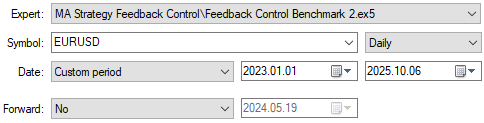
Рисунок 11: Установка эталона оптимизации с помощью нашего линейного регулятора с обратной связью
Система переходит от постоянных убытков к стабильной прибыльности. Точность повышается с уровня около 45% до более 50%, в то время как количество сделок сокращается, что свидетельствует о повышении эффективности. Наши показатели коэффициента Шарпа и коэффициента восстановления значительно улучшились. И все эти улучшения были реализованы без того, чтобы мы явно указывали приложению, что именно оно должно делать для повышения производительности.
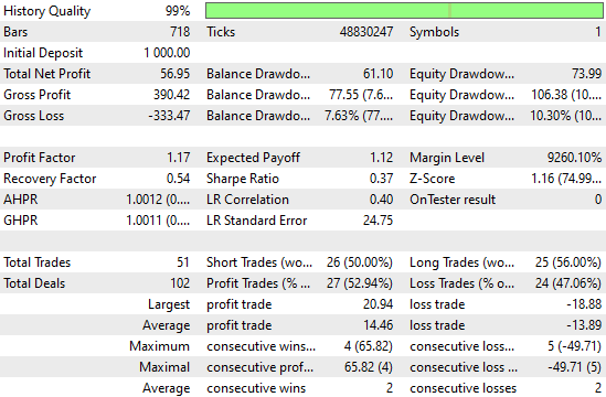
Рисунок 12: Подробный анализ улучшений, достигнутых благодаря линейной системе, которую мы определили на основе зарегистрированных нами наблюдений
Новая кривая капитала заменяет прежнюю нестабильность устойчивым ростом, и ранние падения больше не повторяются в последующие периоды. Даже во время серий убытков система никогда не падает так низко, как раньше.
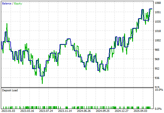
Рисунок 13: Визуализация кривой капитала, сгенерированной усовершенствованной версией нашего торгового приложения
Заключение
На этом мы заканчиваем наше сегодняшнее обсуждение. Мы полагаем, что эта статья продемонстрировала вам, как с помощью API MQL5 можно расширить возможности регуляторов с обратной связью за счет машинного обучения, чтобы справляться с неопределённостью, повысить эффективность использования капитала и стабилизировать торговые системы на волатильных или меняющихся рынках. Читатели получат четкое представление о том, почему традиционные стратегии зачастую оказываются неэффективными и как их можно систематически совершенствовать с помощью методов, основанных на данных, а также ознакомятся с практическими способами внедрения регуляторов с обратной связью, оптимизации показателей и управления рисками. В конечном итоге, представленные концепции позволят вам превратить нестабильные или неэффективные стратегии в управляемые и прибыльные системы.
| Название файла | Описание файла |
|---|---|
| Feedback Control Benchmark 1.mq5 | Классическая версия стратегии, результаты которой мы стремились превзойти, анализируя её взаимосвязь с рынком. |
| Feedback Control Benchmark 2.mq5 | Мы реализовали регулятор с обратной связью, чтобы выявить взаимосвязь между нашей стратегией и текущей рыночной конъюнктурой. |
Перевод с английского произведен MetaQuotes Ltd.
Оригинальная статья: https://www.mql5.com/en/articles/19891
Предупреждение: все права на данные материалы принадлежат MetaQuotes Ltd. Полная или частичная перепечатка запрещена.
Данная статья написана пользователем сайта и отражает его личную точку зрения. Компания MetaQuotes Ltd не несет ответственности за достоверность представленной информации, а также за возможные последствия использования описанных решений, стратегий или рекомендаций.

- Бесплатные приложения для трейдинга
- 8 000+ сигналов для копирования
- Экономические новости для анализа финансовых рынков
Вы принимаете политику сайта и условия использования